


All Issues
Stress-adapted landscapes save water, escape injury in drought
Publication Information
California Agriculture 45(6):19-21.
Published November 01, 1991
PDF | Citation | Permissions
Abstract
Results of investigations at UC experiment stations reveal that irrigation equal to 14% or less of reference evapotranspiration (ETO) can be applied to established shrubs and ground covers with no apparent drought-related injury. Adaptation to stress by reduced irrigation during the 2 years preceding full reduction of irrigation eliminated most injury symptoms (such as wilting and leaf necrosis). Application of these findings to established landscapes should significantly reduce water use and the cost of removing excess vegetation.
Full text
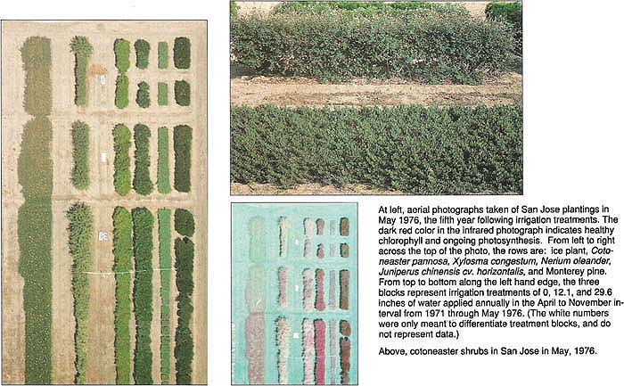
At left, aerial photographs taken of San Jose plantings in May 1976, the fifth year following irrigation treatments. The dark red color in the infrared photograph indicates healthy chlorophyll and ongoing photosynthesis. From left to right across the top of the photo, the rows are: ice plant, Cotoneaster pannosa, Xylosma congestum, Nerium oleander, Juniperus chinensis cv. horizontalis, and Monterey pine. From top to bottom along the left hand edge, the three blocks represent irrigation treatments of 0, 12.1, and 29.6 inches of water applied annually in the April to November interval from 1971 through May 1976. (The white numbers were only meant to differentiate treatment blocks, and do not represent data.)Above, cotoneaster shrubs in San Jose in May, 1976.
The current prolonged drought suggests that California is unlikely to enjoy an inexpensive water supply in the future. Moreover, reduced water use in all areas of landscape management not only makes economic sense but will likely be mandated by legislation. Design and installation of drought-tolerant and perhaps more salt-tolerant landscapes with careful water management should become commonplace as more information on the minimum water requirements of representative environments becomes available. This is a report of past research on the subject where the objectives were to determine the minimum irrigation required to maintain healthy-appearing plants and to develop techniques for estimating when established plants require irrigation.
From 1971 through 1974, hedgerow plantings of Ligustrum lucidum (glossy privet), Pittosporum tobira (tobira), Nerium oleander (oleander), Coprosma baueri, Xylosma congestum, Eugenia uniflora, Hedera (Algerian ivy) and Carpobrotus (ice plant) at UC experiment stations at Irvine (Orange County) and San Jose (Santa Clara County) were subjected to low irrigation regimes calculated as a fraction of reference evapotranspiration (ETo). ETo approximates the amount of water evaporated from a large field of an adequately irrigated, 4- to 6-inch-tall cool-season grass. (For complete definition, see Fulton et al., p. 38, California Agriculture, September-October 1991.) The hedgerows and ground covers were established at experiment stations in San Jose and Irvine in 1965. Six years later, the plantings were subjected to three or four different irrigation regimes: (1) replacement ETo, (2) one or two irrigations beginning 30 days following the last significant rainfall (see figs. 2 and 3), and (3) no irrigation. At both San Jose and Irvine, no significant rain fell after March 1974; all water was provided to plants via irrigation systems. All irrigation treatments began with the soil profile wet to a depth of 4 feet (ft). The experiments were not replicated.
Irrigation was by row and furrow with 3 to 4 inches applied at each irrigation. Water applications were not as uniform as they would have been if drip emitters had been used (more water penetrates the soil at the head of the furrow). More water was undoubtedly lost to evaporation than would have been the case in a drip system. The volume of water applied was calculated from the rate of flow of water from the irrigation pipe and the duration of each irrigation. Soils were well-drained, sandy loams that were wet to a depth of 4 ft by each irrigation. Current research at Irvine, in cooperation with San Diego County Farm Advisor David Shaw, essentially repeats the earlier research, with the exception that an automated drip irrigation system has been installed and soil moisture sensors are set at a depth of 2 ft.
To convert acre-inches (ac-in) to gallons (gal), when irrigation is applied to a landscape of known area, the following information is required: 1 ac-ft = 325,900 gallons, 1 ac-in = 27,153 gallons and 1 ac = 43,500 ft2. Therefore, 4 ac-in applied to a 1000 ft2 plot would be 1000/43,500 x 4 x 27,153, or approximately 2,500 gallons (0.62 gal/ft2=l ac-in).
Test site evapotranspiration
Records of evaporation from open pans of water are kept at all weather stations in California. From these data, ETo is computed and tables of ETo are available for most locations. (For added details on ETo see Snyder, R. L., W. O. Pruitt and D. A. Shaw, 1984, Determining Daily Reference Evapotranspiration (ETo), Leaflet 21426, Cooperative Extension, UC Division of Agriculture and Natural Resources, UC Davis.) We used 10-year average records to calculate water deficits experienced by the plants in the different irrigation regimes at Santa Ana and San Jose. The average values are so close to those for individual years that they are sufficiently accurate to interpret the experiments performed during 1973-74. However, real-time numbers should be used in irrigation scheduling.

Fig. 1. Growth of shrubs at Irvine as a function of irrigation water received from March through September 1974. No black bar appears for “0 inches irrigation” because no growth occurred under this condition. Rainfall during the winter of 1973-74 was 10.9 inches. All but the nonirrigated plants retained an acceptable appearance for landscape purposes.
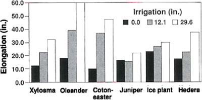
Fig. 2. Growth of shrubs at San Jose as a function of irrigation water received from March through September 1974. The 12.1 in. were applied in three irrigations in May, July and September; the 29.6 in. were applied in eight irrigations at 2-week intervals beginning in April.
In the third year after the beginning or the irrigation treatments, by which time the plants in the zero- and low-irrigation regimes were “hardened,” growth data were recorded. From May through September of 1974 in Santa Ana and San Jose, the periods for which growth and appearance data were recorded, the cumulative ETo was 30.4 inches at the South Coast Field Station and 29 inches at San Jose.
Growth of plants
The data in figures 1 and 2 show that vegetative growth was reduced substantially in 1974 in the low-irrigation treatments, so that the shrubs in these treatments would not have required pruning (no vegetation removal). Less than 4 inches of irrigation water, approximately one-eighth of the ETo, was required to maintain shrubs in a healthy condition. All species retained an appearance suitable for most landscape purposes. Only the nonirrigated shrubs at Irvine suffered significant leaf loss; their appearance was not acceptable. Yet the single irrigation in May, supplying 3.7 inches of water, was adequate to maintain plants in excellent condition. At San Jose, all species grew and retained excellent appearance without irrigation. Note that rainfall at San Jose was 5 inches greater during the winter of 1973-74 and ETo somewhat lower than at Irvine.
Not only was growth during the 1974 growing season reduced, but the leaf area of the zero- and low-irrigated plants was significantly reduced from 1971 to 1974, the period of adaptation. Before 1971, all of the plants were grown with near replacement ET, that is, at their maximum growth rates. Hence, they developed lush canopies, which required substantial pruning (see the growth data for the 29.6-inch irrigation regime).
Remote sensing: leaf temperature
Can remote sensing of leaf temperature be used to estimate irrigation needs in nonirrigated plants? Leaf temperature has been used to measure moisture stress and irrigation requirements in some landscape and crop species, but has not been applied to systems where only minimum growth and satisfactory plant appearance are desired. To determine whether leaf temperatures could be used to estimate when irrigation is required, a remote-sensing, thermal-imaging system was used to measure leaf, air and soil temperatures. Plants at San Jose that were not irrigated were generally warmer than those that were irrigated (fig. 3). Ice plants were up to 25°F warmer than the surrounding air when air movement was minimal, less than 5 miles per hour (mph). With wind velocities above 5 mph, leaf temperatures in the nonirrigated ice plants were close to ambient air temperature. Hence, the leaf temperature method of measuring stress would not be useful in most areas of California where wind velocities are frequently greater than 5 mph unless the relationship between wind velocity and leaf temperature were known with some precision. Xylosma foliage, further above the ground, with thinner leaves that dissipate heat by conduction and convection more rapidly than those of ice plant, were only 10°F warmer than the surrounding air when air movement was less than 5 mph.
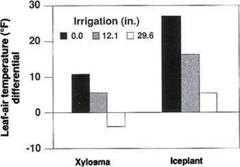
Fig. 3. Leaf-air temperature differentials for San Jose xylosma and ice plant as a function of irrigation regime. Temperatures were measured July 26, 1974, using infrared imaging system. Air temperature was 76°F.
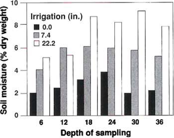
Fig. 4. Soil moisture as a function of depth and irrigation regime at Irvine. Cotoneaster plants extracted water from at least a 3-ft depth in the nonirrigated block (these shrubs suffered excessive leaf damage). Measurements were taken in October, 1974; rainfall in 1973-74 was 10.9 inches.
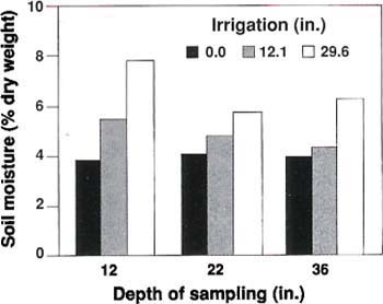
Fig. 5. Soil moisture as a function of irrigation regime at San Jose, sampled at 12, 22 and 36 inches. All shrubs appeared healthy. Sampling below Xylosma plantings was done on September 16, 1974. Rainfall in 1973-74 was 15.2 inches.
Soil moisture, rooting depth
The well-irrigated shrubs at Irvine and Santa Ana had an average rooting depth of 4 to 6 ft. The soil profile was wet down to at least 4 ft at the beginning of the irrigation trials in April. No quantitative estimates were made, but the bulk of the root systems in the nonirrigated and very infrequently irrigated blocks was in the upper 2 to 3 ft. Below this level, roots were not apparent although fine roots would have escaped attention by the coarse methods used.
Soil moisture was extracted down to at least 3 ft in all irrigation treatments at Irvine and San Jose (figs. 4 and 5, sampling in September and October 1974) and was below 5% in the nonirrigated plots. Tensiometer readings for the monthly irrigated plots were -40 to -60 centibars. In nonirrigated blocks, readings were not determined because they fell below -80 centibars, a region where tensiometers are not accurate. Different kinds of sensors are required to control irrigation systems where minimum irrigation is desired and soil moistures are routinely in the 3 to 5% range. Current research at Davis involves testing and calibrating newly available electronic sensors at soil moistures below 5%.
Sensor placement
In a drip irrigation system with emitters irrigating only a portion of the root system, we believe that sensor placement is critical. Current experiments with oleander and pittosporum shrubs suggest that a capacitance-type sensor placed at the one-foot level of the root zone, about 1 ft from an emitter, is an effective system regulator.
Rooting depth as a function of plant size and soil type
More frequent irrigations of shorter duration than used at San Jose and Irvine are recommended if the effective rooting depth of the plants is less than 3 ft. This is often the case for small perennials. Also, in heavy clay or compacted soils rooting depths may be less than 3 ft owing to restricted oxygen supply.
Stress-adapted landscapes save water, escape injury in drought