


All Issues
How will changes in global climate influence California?
Publication Information
California Agriculture 63(2):59-66. https://doi.org/10.3733/ca.v063n02p59
Published April 01, 2009
PDF | Citation | Permissions
Abstract
In 2007, the Intergovernmental Panel on Climate Change (IPCC) published its fourth assessment reports summarizing recent global climate change and projections for the next century. This article reviews the basics of climate science and modeling, highlights the conclusions of the IPCC report, and identifies the well-understood aspects of climate change that will be important for California agriculture and society as a whole. Predicted impacts to California include increased flooding and reduced water availability, higher sea levels, worse air pollution and fewer chilling hours for important crops.
Full text

In a warmer world, the availability of water is likely to be the most important issue that Californians face. Reservoirs such as Shasta in Northern California, shown in fall 2008 at nearly 60% of its capacity, will likely be fuller in winter, and lower in spring and summer when crops are irrigated.
Important consequences of observed and future global warming are as diverse as decreases in winter chilling hours (a necessity for many fruit and nut crops), more extreme air pollution episodes and more frequent coastal flooding. Most important are past and future reductions in winter snowpack, which increase the likelihood of winter flooding, and reduce the water available from reservoirs for irrigation and other uses in late spring and summer.
During the past decade, the most controversial subject in atmospheric science has been the question of whether humans are having a significant impact on climate. The Intergovernmental Panel on Climate Change (IPCC) recently evaluated many aspects of global climate change in a set of extensive reports. These reports are compiled by panels of hundreds of scientists and social scientists from around the world under the umbrella of the United Nations. They describe comprehensive evaluations of the published literature concerning global climate change. The Physical Science Basis report alone is nearly 1,000 pages, and establishes the basis of climate science and the most recent climate observations and model results (IPCC 2007). This review of the IPCC report and other recent scientific literature focuses on the most important factors that influence agriculture in the western United States.
The science of climate
We put the IPCC conclusions into context using the basics of climate change science (fig. 1). In general, the temperature of Earth's atmosphere is determined by a balance between the amount of trapped sunlight and the nearly equal loss of heat into deep space. The distribution of sunlight and that the equatorial regions are warmer than the poles, and that summer is warmer than winter. Atmospheric winds and ocean currents further influence the mean climate. For instance, the U.S. West Coast is relatively mild in winter because warm ocean air flows from west to east. However, in summer that oceanic flow is relatively cool partly because the Alaska current cools coastal waters.
For Earth, the amount of trapped sunlight during a year is closely offset by a nearly equal amount of heat being lost into deep space. However, global climate change will occur if, over years or decades, either the amount of absorbed sunlight or emitted heat changes. The amount of absorbed sunlight varies for a number of reasons, including slight fluctuations in solar output, changes in cloud cover and variations in snow cover. The two latter factors alter what is known as Earth's “albedo,” the fraction of sunlight that is reflected back into space. In addition to natural factors, the amount of absorbed sunlight may be altered by human activities. For instance, we may increase the surface albedo by replacing black asphalt with more reflective, light-colored concrete, or the top-of-atmosphere albedo through introduction into the atmosphere of reflective aerosols (dust particles), primarily as a result of burning fossil fuels. Both of these factors will lead to decreased absorption of solar radiation at the surface and lowered surface temperatures.
Greenhouse effect.
Changes in the greenhouse effect are the primary ways that humans can influence climate.
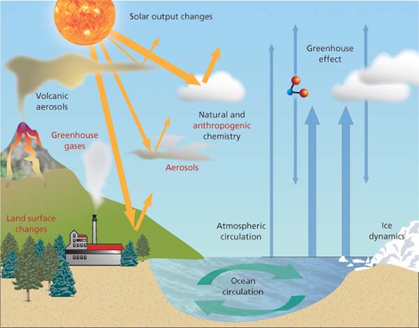
Fig. 1. Schematic of factors and processes controlling global climate; the primary controls are changes in solar radiation (yellow arrows) and outgoing heat (blue arrows). Adapted from IPCC 2007, fig. 1.2.
Each greenhouse-gas molecule can absorb a tiny portion of upward-traveling heat (fig. 1), which it must release almost immediately. This release occurs in all directions, so that part of the heat, which was originally leaving the atmosphere, is redirected back down to the ground. This means that less heat escapes to outer space and more heat heads toward Earth, increasing surface temperatures.
The major constituents of the atmosphere, nitrogen and oxygen, absorb almost no heat or sunlight. Their concentrations have little direct effect on climate change. The main naturally occurring greenhouse gases are water vapor and carbon dioxide. Without these gases the average surface temperature of Earth would be about 32°F (18°C) cooler than today — not a very pleasant place. Humans can add to the greenhouse effect by emitting carbon dioxide, mostly from the burning of fossil fuels, and other greenhouse gases such as chlorofluorocarbons, methane and nitrous oxide.
Feedbacks.
An initial temperature change due to radiative factors may be amplified or diminished by positive and negative feedbacks (fig. 1). An example of a positive feedback is the snow-albedo feedback mechanism, which an initial increase in temperature leads to less snow and ice at higher latitudes. Since both ice and snow easily reflect sunglight back to space, this decrease will lead to more sunlight being absorbed by Earth's climate system, tending to increase the temperature even more. Another well-understood positive feedback is related to water vapor, the most important greenhouse gas. As Earth warms, the ability of the atmosphere to hold water vapor generally increases. The additional water vapor absorbs more heat and causes Earth to warm further.
Negative feedbacks may also occur, which tend to reduce the magnitude of the overall temperature change but not its direction. For example, in the moister atmosphere associated with higher temperatures, thicker clouds are likely to form. Increased cloud thickness will lead to lower surface temperatures, primarily because clouds effectively reflect sunlight. The initial temperature increase may therefore be reduced.
2007 IPCC Report
The recent IPCC report concludes that warming of the climate system is “unequivocal,” that this warming is “very likely” due to increased anthropogenic greenhouse-gas concentrations, and that continued greenhouse-gas emissions and climate changes are “very likely” to be larger in the next century. Some important details of the IPCC report are discussed below; quotations from the report are shown in italics.
Climate-forcing factors.
Global atmospheric concentrations of carbon dioxide, methane and nitrous oxide have increased markedly as a result of human activities since 1750 and now far exceed preindustrial values determined from ice cores spanning many thousands of years … The primary source of the increased atmospheric concentration of carbon dioxide since the pre-industrial period results from fossil-fuel use, with land-use change providing another significant but smaller contribution. The atmospheric concentration of methane in 2005 exceeds by far the natural range of the last 650,000 years (320 to 790 parts per billion [ppb]) as determined from ice cores. The global atmospheric nitrous oxide concentration increased from a preindustrial value of about 270 ppb to 319 ppb in 2005.
Although atmospheric carbon dioxide concentrations have increased steadily, only about half of the fossil-fuel-related carbon dioxide released into the atmosphere over the past century has remained there. The other half has been deposited primarily into the deep oceans and terrestrial bio-mass — forests and soil humus. The increasing concentrations of methane are believed to be largely related to natural-gas drilling and distribution, feedlot emissions and decomposition in landfills and rice fields. Increases in nitrous oxides are primarily related to air pollution and livestock waste management (see page 79).
Increases in these and other anthropogenic and natural climate-forcing factors result in changes, which can be related to an equivalent change in the solar heating of Earth. Figure 2 (page 62) illustrates the current values of most of these factors and uncertainties in the estimates. The most important forcing factors, having the lowest relative uncertainties, are positive and lead to global warming. However, other anthropogenic climate-forcing factors, which have estimated influences that are relatively uncertain, are leading to a smaller amount of cooling. Natural variability of the sun currently is also inducing slight heating (fig. 2). Another possibly relevant natural cooling factor, not shown in figure 2, is the unpredictable but important effect of strong volcanoes, which put large amounts of aerosols (reflective dust particles) in the stratosphere, resulting in less solar heating and leading to a cooling of Earth's surface for up to a few years.
Magnitude of warming.
Warming of the climate system is unequivocal, as is now evident from observations of increases in global average air and ocean temperatures, widespread melting of snow and ice, and rising global average sea level. The overall temperature increase has been about 1°F (0.5°C) over the past century. The warming is largest over the highest latitudes and the centers of continents and smallest over the tropics and the oceans.
Sea level.
Global average sea level rose at an average rate of 1.8 millimeters (0.07 inch) per year from 1961 to 2003. There is high confidence that the rate of observed sea-level rise increased from the 19th to the 20th century. The total 20th-century rise is estimated to be about 0.17 meter (6.6 inches). Most of this increase in sea level is thought to be due to the expansion of water in the oceans as they warm. Another fraction, whose magnitude is subject to considerable debate, is due to the increased melting of mountain glaciers and of small fractions of the massive ice of Greenland and Antarctica.
Role of greenhouse gases.
Palaeo-climatic information supports the interpretation that the warmth of the last half-century is unusual in at least the previous 1,300 years. Most of the observed increase in global average temperatures since the mid-20th century is very likely due to the observed increase in anthropogenic greenhouse-gas concentrations. This is a stronger, more conclusive statement than was made in the previous IPCC report, which was released in 2001. In fact, the current report concludes:
The observed widespread warming of the atmosphere and ocean, together with ice mass loss, support the conclusion that it is extremely unlikely that global climate change of the past 50 years can be explained without external forcing, and very likely that it is not due to known natural causes alone.
For the next two decades, a warming of about 0.2°C (0.4°F) per decade is projected for a range of SRES (Special Report on Emissions Scenarios) (Nakićenović and Swart [2000]) emissions scenarios (discussed below). Even if the concentrations of all greenhouse gases and aerosols had been kept constant at year 2000 levels, a further warming of about 0.1°C (0.2°F) per decade would be expected. Continued greenhouse-gas emissions at or above current rates would cause further warming and induce many changes in the global climate system during the 21st century that would very likely be larger than those observed during the 20th century.
The overall conclusion of this IPCC report is that there will likely be a steady increase in global, hemispheric and regional temperatures in the next century due to human influences. The magnitude of the changes will largely depend upon future increases in greenhouse-gas emissions and, perhaps, changes in anthropogenic aerosol concentrations resulting from a broad variety of human activities.
Global climate models
Global climate models are the most important, and probably the most widely misunderstood, tools used by climate scientists to understand past climate changes and estimate those of the future. State-of-the-art, physics-based computer models are an outgrowth of weather models, which are used to make forecasts 1 to 10 days into the future. Although we all sometimes make fun of weather forecasts, it is now possible to forecast 4 days with the same accuracy as it was possible to forecast 3 days a decade ago.
Glossary
Albedo: Fraction of sunlight at the top of the atmosphere that is reflected back into space.
Albedo, surface: Fraction of sunlight hitting a surface (such as a polar icecap, cropland or resurfaced parking lot) that is reflected upward.
Emissions scenarios (A2, B1): The A2 (high emissions) economic scenario assumes relatively rapid global population and economic growth with few controls on fossil-fuel emissions. The B1 (lower emissions) scenario assumes extensive emissions controls such that atmospheric carbon-dioxide concentrations do not exceed 550 parts per million (ppm), less than 50% higher than the current value of about 380 ppm.
Feedback, positive and negative: A sequence of processes, which will either amplify (positive) or reduce (negative) the size of an initial change, such as a surface temperature increase. Generally a negative feedback will not alter the sign of the change.
Forcing factors: Factors external to the natural ocean-atmosphere climate system that greatly influence climate. Natural forcing factors include output of the sun (radiant energy) and volcanic aerosol (dust) concentrations. Human (anthropogenic) forcing factors include concentrations of greenhouse gases such as carbon dioxide and methane.
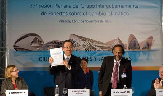
In November 2007 in Valencia, Spain, United Nations Secretary-General Ban Ki-moon (center), flanked by Renate Christ (left), secretary of the Intergovernmental Panel on Climate Change (IPCC), and Rajendra Kumar Panchauri (right), IPCC chair, displayed the fourth IPCC assessment report, which concluded that warming of the climate is “unequivocal.”
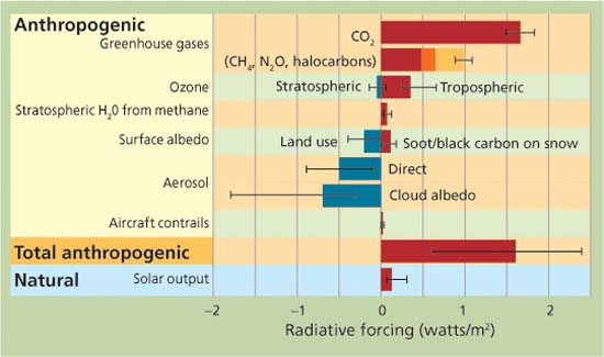
Fig. 2. Primary forcing factors for global climate change. Magnitudes are expressed in terms of the equivalent change of incoming sunlight at the top of the atmosphere. The temporary cooling effect of unpredictable, massive volcanoes is not shown. Adapted from IPCC 2007, fig. SPM.2.
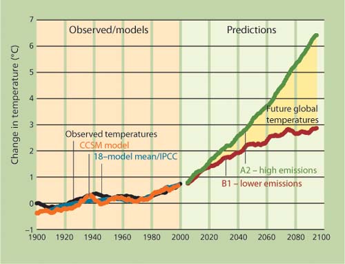
Fig. 3. Observed and predicted changes in average surface temperatures in the Northern Hemisphere. Observed/models (left) shows: observed temperatures between 1900 and 2000 (Mitchell and Jones 2005); 18-model mean sample of IPCC global ocean-atmosphere predictions starting about 1850, for 1900 to 2000; and Community Climate System Model (CCSM) prediction for 1900 to 2000. CCSM predictions (right) for 2000 to 2100 are based on the A2 (high emissions) and moderate B1 (lower emissions) economic scenarios. The likely range of global temperatures in the future is between the green and red lines.
Modeling climate processes.
The procceses simulated by these climate models (fig. 1) involve the physics not only of the atmosphere, but also oceans, ice masses and land surfaces. To emulate these processes in the atmosphere, the models calculate the temperature, pressure, winds and humidity at points between 50 and 150 miles apart in the horizontal direction and as much as a few thousand feet in elevation. At each point, the models mathematically solve the basic laws of physics, including Newton's laws of motion, the conservation of energy and the conservation of total mass and water. Comparable calculations are made for the oceans to predict area-averaged currents, temperature and salinity.
These large-scale processes are coupled to carefully tested approximations of subgrid-scale processes, which occur in regions that are smaller than the spacing of most model grids. An example is the interaction of atmospheric temperature and winds with clouds, which individually occur over regions of a few hundred yards to a few miles, but which also as a group are vitally important for determining the global climate. Other subgrid-scale processes include turbulence near the ground, the growth of cloud drop to rain drops, land-surface interactions, and in some climate models, atmospheric and oceanic chemistry, and plant growth.
How models work.
To use a climate model one starts with the observed conditions for one time in the past, than all of the relevant equations are projected into the future in intervals of a few minutes. The primary controls on climate are basic physics and forcing factors such as solar output and greenhouse-gas concentrations. This process creates descriptions of day-to-day weather a year or decades into the future. After many thousands of time steps, estimates of nearly any climatic variable for some future time, such as 50 years from now, can be obtained from averages of the appropriate output. The development of a climate model that simulates future weather is somewhat like making homemade ice cream in a churning ice cream maker. The ice cream ingredients correspond to the composition and structure of the atmosphere/ocean/ice system. The stirring rate of the ice cream maker corresponds to Newton's laws of motion, and the temperature corresponds to the climate-forcing functions, such as sunlight received at the top of the atmosphere. The hardness and consistency of the ice cream at any time is equivalent to Earth's weather. As the ice cream maker turns, the cream mixture evolves by becoming harder and smoother. As a climate model evolves, that is, moves forward in model time, it makes predictions of temperature, precipitation and other variables further and further into the future. Just as in the ice cream maker, where the final product is primarily a function of the ingredients and mixing of the maker, in a climate model the final climate is primarily a function of the forcing variables and the basic laws of physics. Most importantly, the output of these models is not adjusted in any way by weather or climate observations after the initial step.
Uncertainties of climate predictions.
The uncertainties associated with climate predictions fall largely into two categories. First, there are complex positive and negative climate feedbacks. Second, relatively large uncertainties surround future greenhouse-gas and aerosol emissions, and thus the magnitude of forcing on the model. These uncertainties are primarily related to economic and social projections of the future global economy and human activities.
Evaluating models.
The IPCC models have been used to simulate the 20th-century climate starting at a date before 1900 and controlled by both known natural and anthropogenic factors, such as solar output, volcanic and anthropogenic aerosols, and greenhouse-gas concentrations. The averaged outputs of (1) 18 of these model runs and (2) the representative Community Climate System Model (CCSM) produced at the National Center for Atmospheric Research in Boulder, Colo., emulate very well the observed changes in Northern Hemisphere temperature (fig. 3). The agreement with actual climate data includes the total change over the past century and the fact that heating was slow for the first third, nearly zero in the middle third and relatively fast for the final third (fig. 3). In the western United States, both the 18-run model mean and the CCSM output perform quite well in emulating the changes throughout the 20th century for surface temperature (figs. 4A-C). Observed temperatures generally increase between 1.8°F and 3.6°F (1°C and 2°C) for every degree Centigrade increase in Northern Hemisphere temperature, with the smallest changes over the ocean. Mean temperature changes in the 18 IPCC models and the CCSM both have slightly smaller values than those observed but a similar geographic pattern.
When modeling local changes in precipitation over the western United States that are associated with the observed rise in Northern Hemisphere temperature (figs. 4D-F), the situation is more complex than for temperature. The observed changes indicate both wetter and drier conditions associated with recent global warming (fig. 4D). In contrast, the 18-model IPCC mean precipitation pattern indicates a broad reduction in precipitation over much of the West (fig. 4E). The CCSM results are different again, showing larger changes and a more varied pattern (fig. 4F). This disparity is not unexpected, since short-term weather forecasts of precipitation are less skillful than those of temperature. This is because precipitation processes are complex and have spatial scales much, much smaller than model grid spacing. These results suggest that models do not yet reliably simulate local patterns of precipitation change.
Loss of Arctic sea ice.
The loss of Arctic sea ice, an important aspect of climate change, has received special attention in the last few years (Serreze et al. 2007). There has been a dramatic, well-documented decline in sea ice such that the coverage in September 200/ was only about 60% of the mean for the preceding 30 years. Reports for September 2008 suggest a slightly smaller decline than in the prior year. Nevertheless, rapid decreases in Arctic ice clearly have important consequences for the positive ice albedo feedback mechanisms. More distressing is the fact that the melting of Greenland and Antarctica seem to have accelerated in a manner not well explained by most models (Min et al. 2008).
Future climate predictions
High and lower emissions scenarios.
The main scientific controversies regarding global climate change concern predictions for the future. These predictions combine socioeconomic scenarios of fossil-fuel usage, farming practices and pollution control with global climate models (fig. 3). The right side of figure 3 illustrates predicted average temperatures in the Northern Hemisphere using the CCSM, utilizing the so-called A2 and B1 socioeconomic scenarios. The A2 (high emissions) scenario assumes relatively rapid global population and economic growth with few controls on fossil-fuel emissions. The B1 (lower emissions) scenaric assumes extensive emissions controls such that atmospheric carbon-dioxide concentrations do not exceed 550 parts per million (ppm), about 50%, higher than the current value of about 385 ppm. The true value of future greenhouse-gas forcing factors is expected to be somewhere between these two scenarios. The CCSM model produces average Northern Hemisphere temperature changes that are within the range of all 18 models in the IPCC evaluation (fig. 3). Average surface temperatures in the Northern Hemisphere are likely to rise between 3.6°F (2°C) and 5.4°F (3°C) by 2050 and as much as 12°F (6.5°C) by the end of the 21st century.

Fig. 4. Sensitivity of (A-C) local surface temperature and (D-F) precipitation to changes in Northern Hemisphere average surface temperature (see fig. 3) in the western United States, under observed and model conditions. Blank areas show statistically insignificant changes.
Regional temperature.
When the CCSM is used to predict changes in surface temperature over the western United States for 2050 and 2095 — using the more-sensitive, high-emissions A2 scenario — the temperature changes are largest over the Rocky Mountains and higher latitudes, and smallest over the southern Pacific Ocean (figs. 5A, 5B). Over California, predicted temperature increases are between 1.8°F and 3.6°F (1°C and 2°C) for 2050 and around 7°F (4°C) for 2095. A good deal of confidence may be given to these results because the CCSM model has a sensitivity similar to the mean of the IPCC models, because of the good agreement between the CCSM with observations over the past century (fig. 4), and because of the similar patterns of change for the two future times.

Fig. 5. Changes in (A, B) surface temperature and (C, D) precipitation for 5 years centered on (A, C) 2050 and (B, D) 2095, relative to 2003 values, based on CCMS model and A2 (high emissions) scenario.
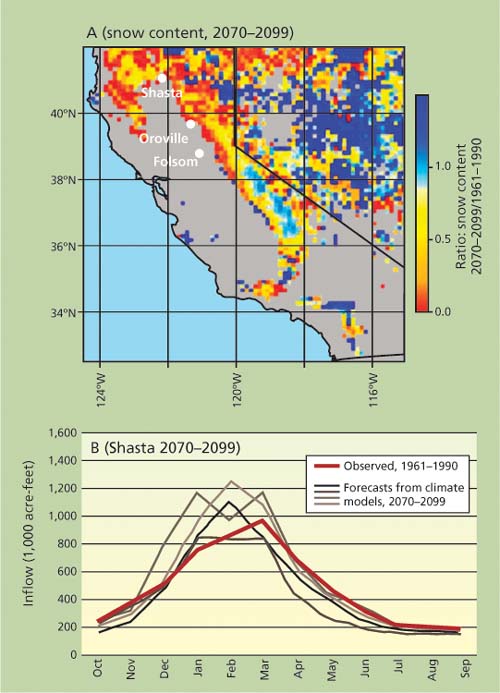
Fig. 6. (A) Ratio of predicted average 2070–2099 April snow water equivalent relative to that observed for 1961–1990. Prediction is based upon a hydrological model driven by the output of a climate model using the B1 (lower emission) scenario. Adapted from Cayan, Mauer, et al. 2008, fig. 14. (B) Monthly mean inflows into Shasta Reservoir for historic period (red line), and output of two climate models each using A2 and B1 emissions scenarios (gray/black lines). Adapted from Purkey et al. 2008, fig. 2.
Precipitation.
When the CCSM is used to predict changes in annual precipitation over the western United States for 2050 and 2095, also using the A2 high emissions scenario, both maps suggest lower precipitation at the lowest latitudes, which is in agreement with other models used in the IPCC evaluation (figs. 5C, 5D). However, the patterns of change over much of the remainder of the region differ from each other and from that of the 20th-century simulations (fig. 4). Unfortunately, little confidence can be placed on local precipitation-change patterns from the CCSM and, perhaps, any current climate model. Because of this uncertainty and because the IPCC climate models generally put the western United States between a broad band of future precipitation increases to the north and decreases to the south, the most reasonable expectation is that total precipitation over the West is unlikely to change substantially from that of today.
Forecasts and California agriculture
Growing conditions.
A number of scientific articles have begun to address what these forecasts mean for California agriculture (see page 55). In addition to the research reported and reviewed in this issue of California Agriculture, a group of articles was compiled in a special edition of the journal Climatic Change (Cayan, Luers, et al. 2008). An earlier summary is given in Hayhoe et al. (2004), with extensive online supplements. Annual mean surface temperatures for California and the western United States are likely to increase substantially in the next century. However, more important to agriculture and society as a whole are variables such as minimum winter temperatures or other extremes. Tebaldi et al. (2006) describe global climate model results for four important temperature statistics: number of days of frost, number of days of the growing season, number of days of heat waves, and percentage of days of warm nights. Their results suggest California will have fewer frost days, longer growing seasons, more heat waves and more warm nights in the future.
Water availability.
Perhaps the most important issues associated with global warming for California are related to water availability. As the western United States warms, mountainous regions will receive rain rather than snow more often and be subject to earlier snowmelt, leading to reduced snow depth and less stored snow water in spring. As a result, there will likely be more flooding, and increased pressure will be placed on the state's reservoir systems.

Fig. 7. Hours in which sea-level height (SLH) is expected to exceed 99.99% of the historical record for San Francisco Bay. Black bars are for all times and red bars are for when sea-level pressure (SLP) is low (during major storm events). Data is based on weather simulations of an ocean/ atmosphere model, adding the influence of a 12-inch sea-level increase. Adapted from Cayan, Bromirski, et al. 2008, fig. 6.
Cayan, Maurer, et al. (2008) predicted the change in April 1 snow content from 2070 to 2099, relative to observed values between 1961 and 1990 (fig. 6). This prediction is based on a snow hydrology model, which is driven by temperature and precipitation values and predicts current snow measurements well. From 2070 to 2099, the precipitation and temperature data are averages from two climate models driven by the moderate B1 (lower emissions) scenario. These models predict increases in surface temperature, but little change in total precipitation (fig. 6A). By 2085 the prediction is the nearly complete loss of April snow at lower elevations of the mountains, substantial losses at middle levels and relatively small losses at the coldest, highest elevations.
Water storage.
Because mountains tend to be conical, losses of low- and mid-elevation snow areas are more important to changes in snow water storage than changes at higher elevations (fig. 6A). For example, flows in Shasta Reservoir are likely to increase in winter, but decrease in spring and summer (fig. 6B). Comparable changes are expected for Oroville and Folsom, which also receive water from mountain regions that are expected to have large decreases in springtime snow (fig. 6A). These changes will tend to raise reservoir inflows and heighten the chances of winter flooding. To offset greater chances of flooding, dam operators will have to reduce reservoir levels. The combined effects of less snowpack and reduced reservoir storage will lead to much less water availability in summer for agricultural and other uses.
Sea level.
Global warming will lead to important increases in sea level, which may influence coastal California. The IPCC report predicts global average sea-level increases by 2060 of 10 to 20 inches (25 to 50 centimeters), leading to increased periods of flooding over the next 100 years (fig. 7). Flooding, which is essentially unheard of in the California of today, may become almost commonplace in the coming century.
Chilling hours.
Baldocchi and Wong (2008) studied hours of chilling, which is important for many fruit and nut crops. Yearly chill-hour accumulation is the number of hours below 50°F (7.22°C). They found that observed chill-hour accumulations over the past 60 years have been variable, but they clearly drop around 1990 (fig. 8). Based on the moderate B1 (lower emissions) scenario, future estimates have realistic year-to-year variability, but also show a clear and substantial downward trend. The number of chilling hours at the end of this century is expected to be half or less than during the 1980s. In this scenario, many crops, such as pears and pistachios, will not be commercially viable in large areas of California where they are currently grown.
Pollution.
Another aspect of warmer temperatures that is likely to affect Californians and agriculture is a projected change in air pollution. The speeds of air-pollution chemistry reactions are often sensitive to temperature and humidity. For example, Kleeman (2008) studied peak concentrations of ozone and small atmospheric particles in the San Joaquin Valley for a period in January 1996, based on a sophisticated air-quality model driven by observed meteorological conditions. When surface temperatures were assumed to increase by 9°F (5°C), peak ozone pollution concentrations were expected to nearly double.
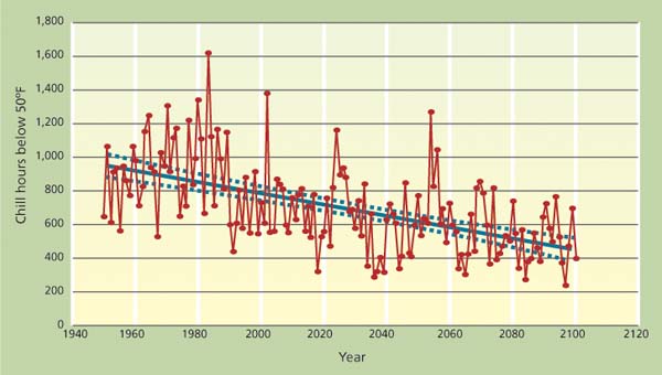
Fig. 8. Past and projected annual total chill hours for Davis, Calif. Values through 2003 are observations; values after are based upon average projections of two climate models driven by moderate B1 (lower emissions) scenario. Adapted from Baldocchi and Wong 2008, fig. 7.
The situation for small particle pollution (PM2.5) is somewhat more complex. Using a similar set of assumptions concerning changes in temperature and humidity, Kleeman (2008) showed substantial increases at the lower elevations of California and decreases in the foothill regions. Even if the emissions rates of pollutants and their precursors remain as today, in a warmer world pollution levels are likely to rise substantially over much of California. These increases could have important detrimental consequences for both natural and managed ecosystems as well as human health.
Human activity and climate change
We now know that relatively large global and regional climate changes have occurred over the past century. Our best scientific evidence strongly suggests that an important component of these changes is due to human activity. Furthermore, persuasive evidence indicates that the changes will continue at an increasing peace well into the next century. Important consequences of observed and future global warming are as diverse as decreases in winter chilling hours, more extreme air-pollution episodes and more frequent coastal flooding. Most important are past and future reductions in winter snowpack, which enhance the likelihood of winter flooding and reduce the water available from reservoirs for irrigation and other uses in late spring and summer.
These changes are likely to have profound influences on all aspects of California's economy and society. Furthermore, the rate of these projected changes will challenge our scientific, economic and social ability to effectively cope. It is important for all Callfornians to understand the causes of these changes, their likely implications and the nature of possible remediation.
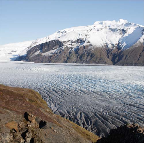
The IPCC found that global sea levels rose 0.07 inch per year between 1961 and 2003, due to warmer oceans and melting of glaciers and polar ice. Above, the glacier Skaftafellsjökull, a spur of the Vatnajökull ice cap, is receding. An August 2008 report by the Icelandic government predicted that Iceland's glaciers will disappear by the middle of the 22nd century.
How will changes in global climate influence California?