


All Issues
Almond advertising yields net benefits to growers
Publication Information
California Agriculture 55(1):20-25. https://doi.org/10.3733/ca.v055n01p20
Published January 01, 2001
PDF | Citation | Permissions
Abstract
This study evaluates the economic impacts of advertising and promotion expenditures funded under the almond marketing order. Over the crop years 1962/63 through 1997/98, the correlation of industry promotion and demand was positive and statistically significant. Almond advertising has yielded marginal benefits between $3 and $10 per dollar spent. The 1994/95 through 1996/97 suspension of the promotion program reduced grower profits in the range of $88 million to $231 million during the suspension period.
Full text
Each dollar spent for almond advertising generates between $3 and $10 of profits for almond growers. Profits fell during the 3-year suspension of the almond promotion program.
The Almond Board of California was established in 1950 by a federal marketing order. The almond order provides the industry with various tools to influence the demand and supply of almonds with the goal of increasing grower returns. Among its provisions, the order authorizes the industry to undertake advertising and promotion. Funds for this purpose are collected through an assessment on almond handlers. The exact provisions of the industry's advertising and promotion program have varied over time, but the order allows, and programs have generally included a provision for, handlers to receive full or partial credit on their assessment for advertising their own products. The industry has also conducted a generic advertising program. The entire advertising program was suspended for crop years 1994/95 through 1996/97 because of litigation.
This study evaluates the economic impacts of advertising and promotion expenditures funded under the almond marketing order and estimates the cost to the industry of suspending its program for the indicated years. Has the advertising program been effective in increasing demand for almonds in the United States, and, if this effect on demand is affirmed, have the expenditures been cost effective in the sense of yielding benefits to growers in excess of the costs borne by them?
U.S. almond consumption
Our study focused on the U.S. market for almonds, where most almond promotion expenditures have been directed. However, because about two-thirds of each year's crop is currently exported, our simulation model takes account of the export market in determining price impacts due to almond promotion. Based on previous studies of the industry conducted by Bushnell and King (1986) and Alston et al. (1995), we specified per-capita quantities of almonds consumed annually in the United States (Qt) as a function of the real (deflated) farm price of almonds (Pt), real consumer income (measured by the per-capita expenditure on all goods, REXPt) and the real annual expenditure on almond promotion (RPROMOt).
We expect the own-price effect to be negative and the income effect to be positive. In other words, an increase in the price of almonds should cause a decrease in almond consumption, while an increase in total money income should lead to an increase in almond consumption. Successful promotions will increase demand, but unsuccessful promotions will have little or no effect on demand.
Given this general specification of U.S. almond demand, the next step was to choose specific functional forms for demand. We limited our consideration to the linear form used by Bushnell and King (1986) and the double-log form used by Alston et al. (1995). The addition of the promotion variable created statistical problems for the double-log model that were not encountered by Alston et al. (1995), whose work did not incorporate this variable. These problems led us to reject the double-log model in favor of a model that is linear in all the variables, except for the promotion variable, which is entered in square-root form. The square-root specification imposes diminishing marginal returns to promotion, meaning that each successive dollar spent yields a smaller incremental benefit than its predecessor. Diminishing marginal returns are necessary or, in principle, it would be optimal to spend an infinite amount on promotion. Here is a mathematical statement of the linear demand model:
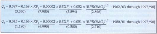
The b coefficients are parameters to be estimated statistically. The term et represents residual changes in per-capita consumption that are not accounted for by changes in the explanatory variables. Because it can be thought of as the error in predicting Qt using only the indicated variables, et is sometimes referred to as the “error” term.
Data for the model consisted of 36 annual observations for crop years 1962/63 through 1997/98. Our measure of promotion expenditures consisted of the sum of the amounts spent on advertising by the Almond Board of California (ABC) and Blue Diamond Growers (BDG), the leading marketer and dominant advertiser of almonds in the industry. For most of the time period we studied, almond handlers like BDG were allowed to satisfy at least a portion of their promotional assessment by advertising their own products. Therefore promotion funded under the auspices of the almond order appropriately includes the amount of assessments credited to BDG and other handlers for the purposes of advertising their own products.

Advertisements like this stimulate demand for almonds.
Because our interest lies naturally in the more recent history of the almond industry, we also estimated the model using the 18 most recent observations available: 1980/81 through 1997/98. It is reassuring if the results based on a shorter time series of more recent data comport with results from analysis based on the full time series. We estimated the model over both the full and the shorter time period using the ordinary least squares methodology (see box below for results).
The numbers in parentheses below each estimated coefficient are t statistics. A t statistic measures the degree of accuracy of the estimate of its associated coefficient. Generally t statistics of 2.0 or more are considered to denote a statistically significant estimate. The effects of price, income and promotion are all significant based on t statistics of 2.0 or more.
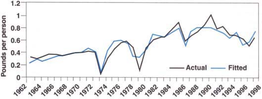
The model estimated for the full sample period explained about 85% of variation in Qt from 1962/63 through 1997/98. The explanatory power of the model estimated over the shorter data set was only 58%, reflecting the greater volatility of the almond industry in recent years. Actual U.S. per capita almond consumption was relatively close to consumption predicted by the model for the 1962/63 through 1997/98 crop years (fig. 1). We also performed several diagnostic tests to check for various statistical problems with the estimated models. Both models passed all diagnostic tests.
The price elasticity of demand evaluated at the means of the full sample was estimated to be approximately -0.7. This elasticity implies that a 1% increase in the price of almonds results in a 0.7% decrease in almond consumption. However, the price elasticity of demand evaluated at the data means for the shorter time series is considerably lower, about -0.35. The difference in elasticity estimates is due to the much larger average consumption for the 1980/81 through 1997/98 period. The greater production and consumption in more recent years has apparently moved the almond industry down along a fairly stable linear demand curve into the more inelastic ranges of the curve.
The promotion elasticities are similar for the two models, about 0.13 for the full sample, indicating that a 10% increase in annual promotion expenditures results (on average) in a 1.3% increase in almond consumption, and 0.15 for the short sample. The elasticities with respect to income are about 0.7 in either instance. Both are in the range of what is considered a “normal” good, in that consumption increases with an increase in income, but the increase is less than proportional. On balance we find that results from the shorter time series compare favorably with results from the full time series, further affirming our belief in the credibility of the estimated model.
Simulation model
Next the estimated model of U.S. demand was used to measure the gross and net benefits to the California almond industry from its expenditures on promotion. The demand models provide estimates of how quantities of almonds sold increase in response to a given increase in promotional expenditures, holding prices and other variables constant. However, price cannot be assumed to remain constant. Indeed, the increase in price following a promotion-induced shift in demand is an important source of the benefits from almond advertising. To properly evaluate the effects of almond promotion, we must combine the estimated demand model with a model of the supply of almonds to the U.S. market.
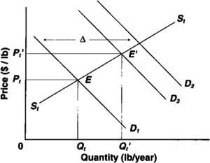
Figure 2 illustrates the conceptual supply and demand relationships for a typical year t. The curve labeled St represents the residual supply curve for almonds to the domestic (U.S.) market. It shows the quantities available to domestic consumers at various prices. At higher prices, more almonds are available domestically; at lower prices, larger quantities of almonds are diverted to other uses, such as to the export market, or they may be left un-harvested or stored across crop years. The curve labeled D1 represents the farm-level demand curve — at higher prices, consumers purchase a smaller quantity of almonds than at lower prices, holding promotion expenditures and other factors constant. The market equilibrium occurs at point E. The market price adjusts until the quantity demanded and the quantity supplied are equated at price P1.
The effect of an increase in successful promotion is illustrated by the outward shift in the demand curve to D2. The econometric model allows us to estimate the horizontal distance of the demand shift in the U.S. market, identified by δ in the diagram. In the model estimated for the full sample, for example, the estimated coefficient on (RPROMOt)1/2 is 0.051. Suppose that the actual annual promotion expenditure is $1 million (in 1998 dollars). This means that a $100,000 (that is, 10%) increase in total promotional expenditures would be expected to lead to an increase in U.S. per-capita almond consumption of 0.051*(1.11/2 - 1.01/2) = 0.0025 pounds per year, if there is no change in price.
Multiplying this amount by the population (267.9 million in 1997/98) yields the total horizontal demand shift in the United States from a 10% increase in promotional expenditures — about a 0.5% increase in average consumption, at constant prices.
However, this is greater than the actual increase in consumption that would result for two reasons. First, an increase in price is needed to bring forth the additional quantities to satisfy the increased demand, as the residual supply curve, St, indicates. Second, an increase in assessments is needed to pay for the additional promotion expenditures. This cost has the effect of shifting farm-level demand down by the amount of the additional per-unit assessment — the curve D3 in figure 2. The new equilibrium is represented by the point E', where D3 intersects St. Price and quantity both increase to Pt′ and Qt′.
To generate a model of the supply of almonds to the U.S. market, we begin by noting that newly planted almond trees do not bear nuts for the first 3 to 4 years. Harvest is therefore determined primarily by yield, which is a function of weather conditions and is largely unaffected by the current year's price. In other words, in the short run (a time window of about 4 years for almonds), price has essentially no effect on total supply. We chose to examine the promotion program over a recent 4-year period so that we could treat bearing acreage as fixed and total harvest as unaffected by the current market price.
The increase in producer profits due to almond promotions under this model formulation is simply the change in the producer price as a result of the promotion multiplied by the amount of the harvest. Further, because supplies are fixed, producers bear the full incidence of the increase in the promotional expenditure. That is, the assessment on handlers will be shifted fully back to growers under this market scenario.
Given our assumptions about supply, the main challenge in the simulation modeling lies in determining the change in producer price due to promotion activities. To estimate this change, the demand model was combined with an assumed residual supply function. This residual supply consists of total supply (assumed to be fixed or inelastic in our model) minus the amount that would be exported at various prices. Given an inelastic total supply, the elasticity, ∊t of the residual supply is found by the formula ∊ = −ηE (QE/QUS), where ηE is the price elasticity of export demand and (QE/QUS) is the ratio of export sales to sales in the U.S. market.
We did not estimate export demand as part of this study, but export demands were analyzed by Alston et al. (1995), who reported values of ηE for Germany, France, the Netherlands, Great Britain, Japan, Canada, Italy and the rest of the world. The elasticity estimates range from a low of −0.43 for Japan to a high of −1.28 for Canada. Assuming a ratio of (QE/QUS) = 2 — that is, about two-thirds of a typical crop is exported — we obtain a lower bound estimate on the residual supply elasticity of ∊L = - (−0.43) * 2 = 0.86 and an upper bound estimate of ∊H = - (−1.28) * 2 = 2.56. Residual supply functions were calibrated using ∊L, ∊H and an intermediate value of ∊ = 1.5. Using this range of values for the residual supply elasticity enabled us to examine the extent to which our results are sensitive to choices of this parameter, where, admittedly, our knowledge is imprecise.

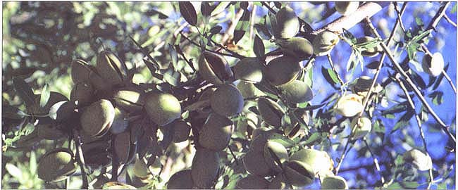
Although most advertising is directed to U.S. consumers, about two-thirds of California's almond crop is exported each year.
By equating the equations for supply and demand and solving for market equilibrium, we obtained values of actual prices and predicted quantities, given the actual values for the explanatory variables REXPt and RPROMOt. We then simulated counterfactual scenarios using a hypothetical, marginal increase in the amount of promotion in each year for 1990/91 through 1993/94 of 1.10 times the actual amount of promotion. We also increased the assessments to pay for that promotion by 1.10 times the actual assessment rate, where we define the “actual” assessment rate as the ratio of total promotional expenditure to the total value of production. Because the program was suspended due to litigation from 1994/95 through 1996/97, the 1990/91 through 1993/94 period represented the most recent 4 years of promotion activity that were in some sense “normal” from the industry's perspective. (We will elaborate on this point in the following section.) The differences between the actual and counterfactual scenarios were then used to calculate measures of the marginal net benefits to producers from the joint increase in promotion expenditures and assessments.
Benefit-cost analysis
Table 1 reports the marginal benefit-cost ratios for almond promotion from 1990/91 through 1993/94 using the alternative values for the residual supply elasticity and the demand models for both the full data set (1962/63 through 1997/98) and the shorter time series (1980/81 through 1997/98). A real discount rate of 3% per year was used to compound the costs and benefits. All monetary calculations are deflated and expressed in 1998 dollars.
The first column in table 1 represents our lower bound, residual supply elasticity of 0.86. In this instance, the benefit-cost ratio for a 10% increase in promotional expenditure based on the full sample is estimated to be 6.88; that is, a marginal $1 expended on promotion yields a return to growers of $6.88. Looking across the columns, we can see the effects of the increase in the residual supply elasticity. As the supply elasticity rises, producers receive progressively smaller benefits from a given demand increase because price rises less for a given demand shift. Therefore the benefit-cost ratio falls from 6.88 to 2.87 when the upper bound, 2.56, of the residual supply elasticity is reached. The range of benefit-cost estimates for the demand model estimated over the shorter time period are greater, due to its more inelastic demand (so that promotion-induced demand shifts generate larger increases in price).
How much confidence can we place in the particular values of the benefit-cost measures? For example, how confident can we be that the benefit-cost ratio is actually greater than 1.0, given a “best” estimate of, say, 3.0. To evaluate the precision of our measures of benefits and costs, we conducted simulations, following the approach developed in Alston et al. (1997). These simulations yield confidence intervals on our benefit measures, permitting us to make probability statements such as that a 95% confidence interval for the benefit-cost ratio is formed by the interval from a:1 to b:1, where a is a lower confidence bound on benefits per dollar expended and b is an upper confidence bound.
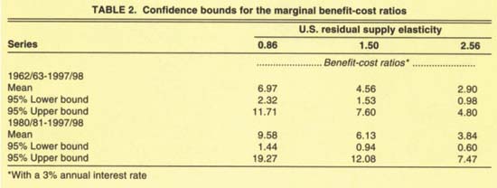
Table 2 provides the mean and lower and upper bounds of 95% confidence intervals for producer benefit-cost ratios from the simulation for each of the residual supply elasticities. For example, the column for a residual supply elasticity of 1.50 in table 2 shows that, based on the demand model estimated over the full sample, the mean from the simulation was 4.56 (which compares closely with the point estimate of 4.51 in table 1) and that a 95% confidence interval for the producer marginal benefit-cost ratio is given by 1.53 to 7.60.

Impacts of program suspension
Suspension of the industry's promotion program from 1994/95 through 1996/97 provides a natural experiment for assessing the impact of the absence of advertising on the almond industry. BDG's promotional expenditures also dropped significantly during this period. The average promotion expenditure by the industry in the 3 years preceding the suspension, expressed in 1998 dollars, was $10.5 million per year, compared with only $3.9 million per year during the suspension.
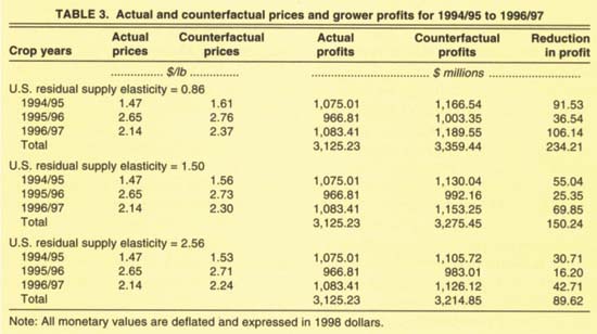
For the 3 years prior to the suspension period, the average effective assessment was $0.02091 per pound (kernel weight). Using this assessment rate with the harvests for the 1994/95 through 1996/97 period would have resulted in the following levels of promotion: $15.3 million in 1994/95, $7.7 million in 1995/96 and $10.6 million in 1996/97. Actual promotion levels were $5.3 million, $4.2 million and $2.2 million, respectively. Using these counterfactual estimates of promotion and the corresponding assessment rate for the years 1994/95 through 1996/97 in the market equilibrium model, allows us to compare estimates of growers' profit obtained using the actual promotion levels and assessments with those obtained under the counterfactual levels.
Table 3 summarizes the results based on the demand model estimated for the full sample. The accumulated loss from the suspension of the promotion program is estimated to be between $89.62 million and $234.21 million, depending on the value chosen for the residual supply elasticity. These estimates are reduction in profit, not just revenue, because the costs of the increased promotion are already accounted for in the model.
Promotion increases profit
Our goal was to evaluate the effectiveness of almond promotions conducted under the auspices of the almond marketing order. The results of the analysis indicate that almond promotion has been a highly effective tool in stimulating almond demand and increasing producer profits. A best guess is that marginal dollars expended promoting almonds have yielded a return to producers in the range of 3:1 to 10:1. Of course, these rates of return are very favorable when compared to returns available to other investments. Given the specifications used in this study, the average return on investments in almond promotion is necessarily higher than the marginal returns noted in table 1.
Suppose, for example, that a 10% rate of return on investment is normal. Then any producer benefit-cost ratio in excess of 1.1:1 indicates a profitable expenditure of funds at the margin. In fact, to maximize its return from investments in almond promotion, the industry should expand promotion efforts to the point where the marginal expenditure on promotion just yields a return comparable to that available on investments elsewhere. Therefore the evidence suggests quite strongly that the industry has spent too little on promotion over the time period analyzed here. Given this evidence, it is unfortunate from the industry's perspective that expenditures were curtailed from 1994/95 through 1996/97 due to litigation. Our analysis suggests that suspension of the advertising program during this period cost the industry accumulated profits in the range of $90 million to $234 million.
Although our focus is on promotion, it is worth noting that this study has also provided some new evidence about the price elasticity of demand for almonds in the United States. The estimates suggest that the elasticity is in the range of -0.35 (shorter time series) to -0.70 (full time series). Therefore the industry is operating in the inelastic portion of its demand curve (at least in the U.S. market), and the large harvests anticipated now and in the future will cause major decreases in producer prices, unless the industry is able to stimulate demand through promotions or other means.
Almond advertising yields net benefits to growers