


All Issues
Optimizing tomato distribution to processors lifts profits little
Publication Information
California Agriculture 49(5):21-26. https://doi.org/10.3733/ca.v049n05p21
Published September 01, 1995
PDF | Citation | Permissions
Abstract
Tomatoes are often hauled long distances in Northern and Central California. Because production areas and processing facilities are not geographically well aligned, processors compete across relatively long distances to procure tomatoes. In this study of the field-to-processor distribution of processing tomatoes, a nonlinear programming model was developed to determine the optimal distribution of tomatoes from the 13 highest-producing counties to the 32 processing plants in the region. Results suggest that excessive interregional haulage of tomatoes occurs, but the additional industry profit from implementing the optimal allocation versus the estimated actual allocation was only 1.9%.
Full text
Older California processing plants lack a significant base of localized production to draw upon and must often source tomatoes from 100 or more miles away. Costs for hauling tomatoes from field to processing facility are 15 to 20% of raw product value.
In 1992 California produced 7.93 million tons of processing tomatoes, over 90% of the U.S. harvest. This harvest generated $447.1 million in plantgate value, making processing tomatoes California's highest valued vegetable crop. Although important and growing, the processing tomato industry is also in a considerable state of flux due to continual changes in the geographic locations and sizes of tomato-producing farms. Urban expansion eliminated processing tomato acreage in many areas and reduced it significantly in others. At the same time, extended irrigation and drainage projects in arid regions such as Fresno County have resulted in marked production increases.
These changes in production are having a profound effect on the processing sector. Processing firms in the San Francisco Bay Area counties now lack a significant base of localized production to draw upon and must often source tomatoes from 100 or more miles away. New processing facilities have been located near the largest concentrations of tomato production, most notably in Fresno County, but in general the processing sector has been slow to follow production.
This geographic evolution of the industry is a dominant force affecting competitive relations among processors and between processors and growers. Nonalignment of production and processing areas has stimulated interregional competition among processors to procure tomatoes and caused tomatoes to be hauled long distances, with hauling costs representing a major expense to the industry. Grower-to-processor transportation costs have averaged from $8 to $12 per ton, or 15 to 20% of the farm value.
We estimate the average one-way haul for California processing tomatoes is about 67 miles, a considerable reduction from the 100-mile haul reported in Brandt, French and Jesse for 1973 (Economic Performance of the Processing Tomato Industry, Giannini Foundation Information Series No. 78-1, UC DANR). Nonetheless, the perception remains among industry participants that tomatoes are distributed inefficiently to processing firms, and that reduced haulage and improved industry performance could be attained if a better grower-to-processor allocation of tomatoes were achieved.
We studied the distribution of tomatoes in Northern and Central California from field to processor and assessed the efficiency of the prevailing allocation pattern. A nonlinear mathematical programming model was developed to determine the optimal allocation of tomatoes from the 13 highest-producing counties to the available processing facilities in the region. With information obtained from the California Processing Tomato Advisory Board (PTAB), we were able to compare the actual allocation with the estimated efficient allocation and estimate losses to the industry from inefficient allocation of tomatoes across processing facilities. Finally, we simulated the introduction of new processing facilities into the industry to study the effect of entry on the distribution of tomatoes among processors.

California's industry
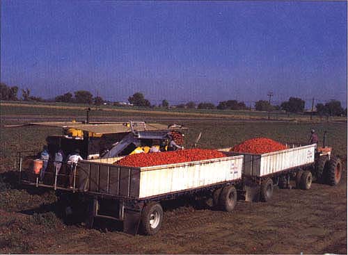
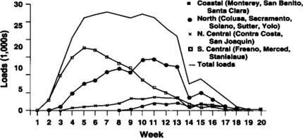
The tomato harvest season lasts about 19 weeks, with the most production occurring between July and September. Harvest begins in the northern-most producing county, Colusa, nearly as early as in Fresno County, over 150 miles to the south. Coastal counties such as Monterey, San Benito and Santa Clara begin production several weeks later. Figure 1 illustrates the 1989 harvest pattern in the major producing regions.
The 13 Northern and Central California counties in this study collectively supplied 88% of the state's processing tomato production in 1989. Figure 2 shows the main producing areas within these counties. While any particular county may spread its production for 10 or more weeks, firms desiring to continue processing operations for longer periods must procure tomatoes from alternative producing areas. Also affecting transportation is the need to ensure even delivery of tomatoes to processing facilities. Plants have incentive to spread purchases across counties so that locally poor yields or damaged crops do not unduly affect processing.
In 1989, the base year of our study, 24 firms operated 37 plants for processing tomatoes in California (compared to 57 plants operating in 1955). Bulk paste accounted for 50 to 60% of processed product output, followed in importance by various sauces, and then by whole peeled tomatoes. Figure 2 indicates the location and type of the 32 processing plants in the study region. Twenty-six plants manufactured diversified products (D), while six plants manufactured only paste (P).
Optimization model
The optimization model was designed to find the weekly allocation of tomatoes that maximized variable profit to the industry, given:
-
The location and characteristics of raw product production by week of harvest;
-
The location, capacity and type of processing plants;
-
Transportation and processing costs; and
-
Selling prices for alternative processed tomato products.
Variable profit to the industry was defined as aggregate revenue from processed product sales, less variable processing costs and transportation costs. Fixed costs of operating the plants are not relevant for short-run industry decision making.
Figures 1 and 2 together provide a good overview of the tomato allocation problem: Production is scattered across much of Northern and Central California and often is not well aligned with the existing processing capacity. The harvest varies significantly by week across the major producing regions and in order for firms to extend their processing season, they must obtain tomatoes from multiple regions.
The data obtained for this study included the number of loads of tomatoes shipped per week from each producing county and the mean and variance of soluble solids among the loads obtained from each county in each week. This information was used to classify each load's content as either high or low in soluble solids. The amount of processed paste, sauce and puree that can be obtained from a ton of raw tomatoes is directly proportional to the solids content of the tomatoes. The production of whole or diced tomato products is not affected by solids content.
The data also included 1989 tomato shipments information for the 32 processing plants located in the study region. These data were gathered under the auspices of the PTAB and are confidential, but permission was obtained to use the data provided that transactions of individual firms were not released. This stipulation meant that shipments data was aggregated into six regional groups of plants (fig. 2) prior to release. Information on the processing capacity of the 32 plants was obtained and verified from a number of sources.
Estimated transportation mileage from each producing county to each processing plant location was based on the available transportation network and the approximate location of production in each county. Transportation costs for each shipment from county to processing plant were computed according to standard truck-rate charges for the industry.
The optimization model also required estimates of processing costs for both paste and diversified-products plants. Production cost data were obtained for a moderately sized diversified-products plant and a paste processing plant, these provided the basic data input for estimating processing plant costs. Through consultations with industry experts, the costs for different plant sizes were extrapolated from the base-line plant costs.
Essentially, the direct labor required in tomato processing operations is constant regardless of the rate of output. However, nonlabor inputs such as cans, cartons, energy, water and various food ingredients such as salt are added to the raw tomato input in approximately fixed proportions. Thus, we considered labor and nonlabor costs separately for both diversified-products and paste plants. Nonlabor costs in both cases were treated as a constant amount per unit of raw tomato processed. Labor costs are the source of nonlinearity in the model because they decline on a perunit basis as a function of the volume of tomatoes processed.
To compute variable profit from tomato processing, we also needed information about the types of processed products being produced. Each firm's product mix is confidential, so the alternative was to assume that the final product breakdown for our base diversified-products and paste plants held across all similar plants. This breakdown was used to construct a composite product to establish the value of a ton of raw tomatoes processed into either diversified or paste products. Costs of canning line operation are quite similar for most canned tomato products, so moderate differences in product mix among processors are unlikely to have a significant impact on per-unit processing costs. (An expanded description of the model is available in our detailed report noted at the end of this article.)
The base optimization problem was to maximize variable profits from processing and selling the 1989 tomato harvest. The problem was subject to the following constraints:
-
A plant cannot process more tonnage than its weekly capacity.
-
A county cannot supply more low-solids (high-solids) tonnage than its low-solids (high-solids) tomato production, in any week.
Formulation and solution of the base optimization model did not involve use of the confidential PTAB inspections data on weekly shipments from producing counties to individual processing regions. This information was incorporated into the program as additional constraints that forced the solution to approximate the actual 1989 allocation. The optimal solution and the constrained optimal solution were then compared and evaluated. The constraint that forces the estimated actual allocation is that:
Optimal vs. actual allocations
In total, 3.73 million low-solids tons and 3.72 million high-solids tons of processing tomatoes were available for allocation in 1989 from the 13 major tomato-producing counties. Table 1 provides an aggregate revenue and cost breakdown comparison for the 1989 solutions to the base model and constrained model.
This comparison reveals evidence of modest inefficiency in allocating tomatoes, as many in the industry have suspected. The optimal solution produces $22.96 million (1.9%) more profit than the model constrained to approximate the actual distribution. The additional variable profit works out to $3.08 per ton of raw tomatoes for the 1989 crop. The average oneway haul in the base model is 56.72 miles, compared to 66.66 miles for the estimated actual allocation. The extra haulage translates into approximately $7.41 million (9.3%) in additional transportation costs borne by the industry under the estimated actual allocation. Based on approximately 290,000 loads of tomatoes harvested from the 13 counties during 1989 and 9.96 average miles of reduced haulage under the base model, we compute that 5.8 million additional round-trip miles were traveled hauling tomatoes in 1989 than if the base model solution had been implemented. Among the 32 processors, 27 incur shorter hauls under the optimal solution than were actually incurred, based on the constrained model solution.
Detailed analysis of the results suggests that the higher transportation costs observed in the constrained model solution mainly were due to misallocations of shipments to processing regions based on county of origin, rather than to aggregate misallocations of tomatoes among processing regions. In other words, inefficient tomato transportation occurs in California because processors do not always procure tomatoes from the lowest-cost production area; it's not that some regions process too many or too few tomatoes. (Note that this conclusion takes the location and magnitude of processing capacity in the industry as given.)
Higher transportation costs accounted for 32% of the higher profits from the base model compared to the constrained model. The rest of the profit gain for the base model came from shipping tomatoes to maximize processing economies in large versus small plants; efficiently allocating high-versus low-solids tomatoes; and expanding relative production of diversified products, which yielded higher profit per ton of raw product than bulk paste did in 1989. In particular, the base model solution allocates 882,000 tons to the six paste-only processing plants versus 1.1 million tons under the estimated actual allocation.
Historically, diversified products such as canned tomatoes have been high-profit items for processors, and our results show a continuation of this tendency. Relatively high profits for diversified products may reflect rents to popular brand names such as Heinz, Ragu or Hunts, or it may reflect the market power of large processors for various processed products. On the other hand, the bulk-paste market represents a classic competitive industry in which the product is basically homogeneous, produced by a large number of California processors and subject to considerable import competition.
The analysis reveals an industry where producers' and processors' fates are closely linked through interregional competition despite being separated, in many cases, by long distances and high transportation costs. Among the 13 major producing counties, eight were estimated to ship tomatoes into five or more of the six processing regions. However, comparison of the optimal solution with the estimated actual tomato allocation indicates that more interregional shipments of tomatoes occurred than was optimal. The base model suggests that more tomatoes should have been processed locally rather than hauled across regions.
Table 2 illustrates these results for the three highest-producing counties. Fresno County in Region 6 attains peak production during weeks 4 through 8 of the harvest, allocating 400,000 or more tons during this time to each of processing Regions 3, 4, 5 and 6 (fig. 2 shows region locations). As the major tomato surplus area, Fresno County ships its tomatoes the greatest average distances throughout the harvest, with an average haul in excess of 100 miles. However, 300,000 tons of Fresno County tomatoes that were hauled north into Region 3 would, according to the base model solution, have been processed more efficiently in Region 4. Similarly 200,000 tons shipped from Fresno County would have been processed more efficiently locally in Region 6.

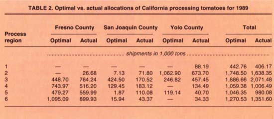
Similarly, in Region 3 approximately 250,000 tons of San Joaquin County tomatoes hauled into Regions 2, 4, 5, and 6 would have been better processed locally; the base model recommends that Region 3 retain its local production rather than import tomatoes from Fresno County.
Parallel conclusions hold for Yolo County in Region 2. Yolo County is the highest producer during the midharvest period, weeks 9 to 13, harvesting nearly 750,000 tons in 1989. Over two-thirds of that production was consumed locally in Region 2 under the optimal solution, with 100,000 tons flowing south to Region 3 and 120,000 tons to coastal processing firms in Region 5, the largest tomatodeficit region. Overall, the base model recommends that 74% of the 1.43 million total tons of tomatoes produced in Yolo County be processed locally — in reality, only about 47% were processed in Region 2. The difference, roughly 400,000 tons, was hauled north into Region 1 (88,000 tons), or south into Region 3 (210,000 tons over the base solution) and Region 4 (134,000 tons). The additional Yolo County tomatoes processed in Region 2 under the optimal solution then allows tomatoes from its southern neighbor, Solano County, to flow into Region 3 rather than stay in Region 2.
Expanding production capacity
We also analyzed the impact on the processing tomato industry of two hypothetical new processing facilities, strategically located in surplus production areas. One plant was located in Region 6 near Madera, along the Fresno-Madera county border, while the other was located in Region 1 in Dunnigan, in northern Yolo County. Both plants were assumed to process diversified products and to have a “large” weekly capacity of 30,000 tons.
Several changes in the base model were implemented to provide the most realistic assessment of the effects on the industry of new entry. First, production levels and locations were updated to 1990 — production in 1990 was 9.3 million tons, somewhat higher than 1989 levels, and may represent a typical production year for the industry. Second, the existing processing capacity in the industry was updated to account for the entry of two new paste processing plants in Region 6 between 1989 and 1990. Finally, the new plant simulations were conducted under a long-run equilibrium assumption whereby paste and diversified-product variable profits were equated, effectively making the choice of paste-only versus diversified-product production for the new plants unimportant.
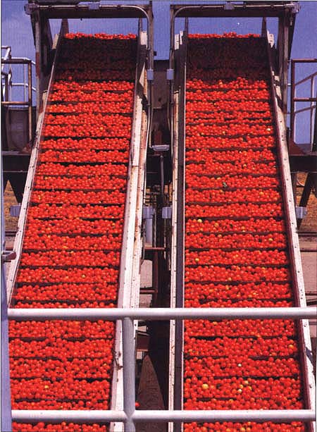
The average one-way haul for California processing tomatoes, shown entering a plant, is about 67 miles. The optimal solution, averaging 56.72 miles, produces 1.9% more profit than the model approximating actual distribution. That works out to $3.08 per ton of raw tomatoes for the 1989 crop.
To assess the impact on the industry of each hypothetical plant, we compared the optimal tomato allocation for the industry for a 1990 base model without either new plant, with the optimal allocation that results when each plant is added to the industry. Despite the addition of the two paste plants in Region 6 in 1990, our analysis suggests that yet another plant in the region would also be a magnet for raw tomato production. Under the optimal allocation, the Madera-area plant operated during weeks 1 through 17 of the harvest season, and operated at capacity for weeks 2 through 13. The plant processed 454,000 tons of tomatoes. The hypothetical plant in Region 1 also attracted a significant volume of tomatoes. It operated in weeks 3 through 13 in the optimal solution with all but the initial week representing capacity operation. Total seasonal tonnage for the plant was 326,500.
The sources of production for the new plants reflect the choices of strategic locations made for them. The Region 6 plant procured its raw tomato supply solely from Fresno County through week 12, at which point it also sourced from Merced, San Joaquin, and/or Stanislaus counties through week 17 (fig. 2). The Region 1 plant was located to give it hegemony over production in Colusa and Sutter counties. Under the optimal solution, this plant was able to procure supply exclusively from Colusa County for weeks 4 to 8 and 10 to 12, drawing tonnage from Sutter County in week 9 and Yolo County in weeks 2 and 13. In total, 95% of the plant's tonnage was obtained from Colusa County.
The new-plant simulations demonstrated that interregional competition to procure tomatoes effectively links processors across Northern and Central California. Entry in one region affects processors in almost every other region. The hypothetical Madera-area plant, although located south in Region 6, affected supply to processors as far north as Region 2 and had significant effects on processors in Regions 3, 4, 5 and 6. The hypothetical northern plant had only a minor effect on total supply allocated to its Region 1 counterparts because Region 1 is a significant surplus producer, but it affected supply to processors in the other processing regions, including the southern Region 6. Whereas 294,000 of the 326,500 tons processed by the Yolo County plant were lost on net outside of Region 1, only 213,000 of the 446,000 tons processed by the Madera-area plant were lost on net outside of Region 6.
These simulation results indicate the comparative vulnerability of processors in the Bay Area of Region 5 and also Region 3 to new competition as a consequence of having to obtain tomatoes from long distances. Region 5 lost 6% of its total tonnage under either simulated entry scenario. This result is particularly striking for the new Yolo County plant because Colusa County, which supplied 95% of its tomatoes under the profit-maximizing allocation, did not supply any tomatoes to Region 5 under the 1990 base model allocation. Instead, the tonnage was lost from Yolo County, where production routed to Region 5 in the base model was allocated to processors that had procured Colusa County production prior to entry of the new plant. The fact that the profit-maximizing allocations for the models with the new plants reduce tomato flows into Regions 3 and 5, relative to the base model allocation, implies that these processors could be outbid for these tomatoes in actual competition by processors exploiting location advantages.
Conclusion
This analysis found modest inefficiency in the distribution of processing tomatoes from farm to processing plants in California and may suggest ways to improve marketing efficiency in the industry through improved crop allocation. Although it may not be feasible, for various reasons, to adopt the optimal solution, some reduction in cross-region hauls indicated by the optimal allocation may suggest profitable alternative contracting opportunities for both growers and processors. However, the results should not be construed as an indictment of present industry practices. Indeed, given all the complicating factors that intervene in the independent production and marketing decisions of nearly 500 growers and 32 processors, it is perhaps remarkable that the variable profit generated by the optimal versus estimated actual allocations differed by only 1.9%.
The study also provides some insights into the nature of spatial competition in the industry. Most counties shipped tomatoes to five or all six processing regions. Simulated entry of new plants at either geographic end of the producing region caused competitive impacts that reverberated across the industry. Our new plant simulations suggest that processing facilities that (1) locate near surplus producing regions and (2) operate at a scale large enough to take advantage of available economies in processing, are capable of performing above the industry norm. Even though existing firms may prefer long-distance hauls to relocation near sources of production as Brandt, French and Jesse have argued, entrants are not constrained by past location decisions. Over time, market forces can be expected to stimulate the creation of these types of facilities, thus causing further restructuring of plant locations and attendant decreases in hauling costs. Such restructuring will occur at the expense of smaller plants located in deficit producing regions.
Optimizing tomato distribution to processors lifts profits little