


All Issues
Proper harvest timing can improve returns for intermountain alfalfa
Publication Information
California Agriculture 56(6):202-208. https://doi.org/10.3733/ca.v056n06p202
Published November 01, 2002
PDF | Citation | Permissions
Abstract
Harvest timing has a profound effect on the yield and forage quality of alfalfa hay. Early harvest results in low yield but high forage quality and price, while delayed harvest increases yield but reduces forage quality and price. Since gross revenue is a function of both yield and price, it is important for growers to select the optimum cutting schedule. We quantified a biological relationship among yield, forage quality and day of harvest, using the results from 2 years of field studies at locations in the intermountain alfalfa production region of California. An economic analysis, including a decision model, was developed to enable producers to assess current market conditions and seasonal effects, and in turn select the most profitable harvest timing. Our analysis demonstrated that no single harvest strategy is always best. The most profitable approach depends on the rate of change in yield and quality for that season and the current price differential between the quality market classes for alfalfa hay.
Full text
The optimal cutting schedule for alfalfa hay is a fundamental concern for alfalfa growers and has been the subject of research for decades (Marble 1980). Alfalfa maturity at harvest affects both the yield and quality of the harvested product Forage quality has a significant influence on price per ton, while yield and price determine the return per unit of land area. Since yield and quality are typically inversely related, determining the most profitable cutting schedule can be a challenge for growers.
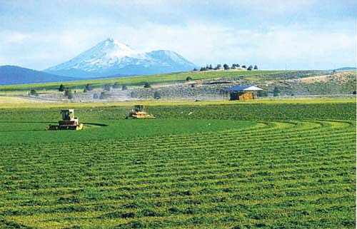
Alfalfa hay is a major California crop, primarily due to the strength of the state's dairy industry. The optimal cutting timing for alfalfa — whether to maximize forage quality (earlier harvest) or yield (later harvest) — is a fundamental concern for growers, including at Prather Ranch, above, near Mt. Shasta.
The demand for alfalfa hay comes from two basic groups, dairy producers and all other users (Konyar and Knapp 1986). California's $4.6 billion dairy industry is the state's primary alfalfa consumer. Alfalfa is an integral component of rations for milking cows and cannot be easily replaced by other feeds. The forage quality or digestibility of alfalfa hay in the dairy ration directly affects milk output per cow. Dairy producers demand alfalfa with high digestibility and protein, and low fiber — particularly for top-producing cows — and they pay extra for this class of hay.
Other users do not need such high-quality hay, and are generally unwilling to pay premium prices. Some classes of livestock, such as beef and nonlactating dairy cows, perform well when rations are balanced with lower quality hay. Horse owners also have quality considerations but their purchasing habits are more visual and physical (for example, they avoid feeds with weeds, mold and/or dust). For this economic analysis, horse demand is included with producers of beef and other kinds of livestock.
For marketing purposes, the forage quality of alfalfa is most commonly expressed in terms of total digestible nutrients (TDN), which is calculated from a lab fiber value (acid detergent fiber [ADF]). While 52% TDN was considered adequate during the 1970s, the market threshold steadily rose during the 1980s and 1990s. Dairy producers now seek 55%, 56% or even 57% TDN alfalfa hay. (TDN is calculated using the California equation, TDN% = 82.38 - [0.7515 x ADF%] and expressed on a 90% dry matter basis.)
Quality affects market value
Forage quality, which determines price, is a continuum with a range of values from high to low. However, there are distinct alfalfa-hay quality designations now recognized by the U.S. Department of Agriculture (USDA) for categorizing hay prices: Supreme (> 55.9 TDN, < 27 ADF, [category created in 1999]), Premium (54.5-55.9 TDN, 27-29 ADF), Good (52.5-54.5 TDN, 29-32 ADF) and Fair (50.5-52.5 TDN; 32-35 ADF). Dairy-quality hay is most frequently associated with the Supreme and Premium grades, and less frequently, with the Good grade; these categories receive significantly higher prices in California than Fair or Low. While the alfalfa market is not as volatile as that for other higher value commodities, the fluctuations are great enough to influence whether alfalfa as a crop option is profitable or not.
From 1992 to 2001, the average annual price for the top category of alfalfa hay from Northern California varied from $89.62 to $136.53 per ton (fig. 1). In addition to price, the quality differential varies significantly from year to year. The price differential — the percentage change between highest category hay (Premium or Supreme] and Fair hay — ranged from 24.4% to 74.3% (expressed as a percent of the lower value) over the same 10-year period.
Yield-quality relationship
Alfalfa yield and quality are inversely related. Harvesting alfalfa at an immature growth stage will result in high forage quality but low yield. Conversely, delaying cutting until a more mature growth stage will result in higher yield but poorer, often unacceptable, forage quality. This presents a dilemma for the alfalfa grower who desires both high yield and high forage quality. Furthermore, little information has been available to assist growers in deciding whether total revenues or profits are maximized with a short or long cutting schedule. This research was undertaken to quantify the yield-quality trade-off in alfalfa and provide tools to determine optimum cutting schedules for the intermountain regions of the western United States.
Field trials were conducted during the first and second alfalfa growth periods, in two high-mountain valleys of Siskiyou County: Scott Valley (elevation 2,700 feet) and Butte Valley (elevation 4,200 feet). Two alfalfa varieties were chosen to represent a range of varieties common to the intermountain region. ‘Blazer XL’, the more dormant variety, has a fall dormancy rating of 3, and ‘Archer' has a fall dormancy rating of 5. The fall dormancy rating is based on alfalfa plant height in fall — lower numbers indicate a more dormant variety.
Alfalfa was harvested every 2 to 3 days, throughout first and second growth periods (late spring and summer, respectively) in 1996 and 1997. A completely randomized design with four replications was used. The first harvest was at the late vegetative pre-bud stage; the last harvest was at full bloom. A different area of each field, with a uniform first-cutting harvest date, was selected for the second-cutting harvests. The total number of harvests per growth period averaged 12, ranging from 9 to 14 depending on the cutting and the location.
Forage yield was measured using a sickle mower from a 3-feet-by-15-feet area of each plot at each harvest date. Each plot was subsampled with eight to 10 randomly selected handfuls of standing crop to determine moisture content and forage quality. Acid detergent fiber (ADF), neutral detergent fiber (NDF) and crude protein (CP) were measured at each harvest using near infrared spectroscopy (NIRS) analysis (NDF and CP data not shown).
Weather conditions during the springs of 1996 and 1997 were very different. Spring 1996 was cool and alfalfa development was delayed approximately 10 days to 2 weeks later than in spring 1997. This illustrates the problem with using a calendar date to time alfalfa harvests. Plant maturity, height and/or other measurements more accurately determine optimal harvest timing. For example, alfalfa harvests at the higher elevation area, Butte Valley, averaged 16 days later than in Scott Valley.
In this study, the location, variety, cutting and year all had significant effects on alfalfa yield and quality changes over time. Location and variety effects, while statistically significant, were small. Our intent was to quantify changes in yield and quality with time rather than to compare varieties or regions, which were included to develop a robust relationship that would hold true across a range of growing conditions in the intermountain region. This relationship would likely differ in areas with widely divergent varieties or growing conditions than those tested.
Quantifying yield, quality changes
As alfalfa matured from the late vegetative pre-bud stage to full bloom, the daily increase in yield per acre for the first cutting was 80 pounds dry matter, averaged over 2 years, two varieties and two locations (fig. 2). In other words, each day delay in the first-cutting harvest resulted in an 80-pound increase in yield. The rate of yield increase was greater for the second cutting, with each day delay resulting in a 112-pound increase in yield.
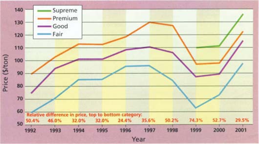
Fig. 1. Average price of alfalfa hay per ton as a function of forage quality for the past 10 years in intermountain regions of California. Percentage is the difference between top and bottom USDA categories, as a percent of the Fair category. (See text for definition of hay quality categories.) The Supreme quality category was added in 1999 (it was combined with Premium in previous years). Source: USDA Market News, Moses Lake, WA.
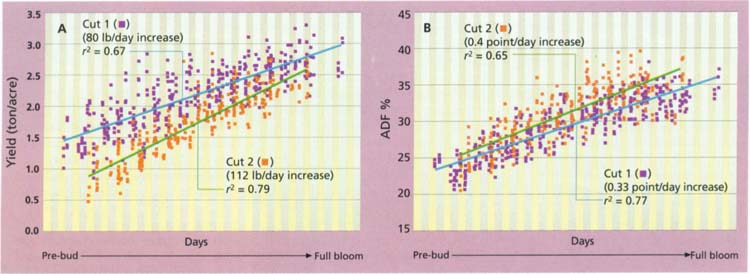
Fig. 2. Relationship between (A) alfalfa yield and (B) acid detergent fiber content (ADF, 100% dry matter), and time of harvest from pre-bud to full bloom for first and second cuttings (over two intermountain locations, 2 years and two varieties). Each vertical column represents 1 day. Lines represent linear regression averaged across locations, varieties and years.
As expected, forage quality declined as the alfalfa matured. During the first growth period, the ADF concentration increased an average of 0.33 percentage points per day. This equates to a loss of 0.22 percentage points of TDN (calculated as a linear function of the ADF value) per day (fig. 2). The increase in NDF per day was very similar to ADF, 0.30 percentage points per day. CP dropped 0.20 percentage points per day on average across locations, varieties and years.
Forage quality declined even more rapidly during the second growth period. The ADF content increased an average of 0.40 percentage points per day on the second cutting. This increase in ADF equates to a 0.27 percentage point loss in TDN per day delay. The NDF concentration increased 0.38 percentage points per day. The average drop in CP on second cutting was 0.34 percentage points per day, declining at a rate 75% more rapid than during the first growth period.
Identifying the optimal cutting schedule for alfalfa hay involves choosing between different price and yield combinations. First, there is the choice of the timing of each cutting, recognizing that delaying a cutting increases the yield but lowers forage quality and thereby price. Second, is the choice of how many cuttings to make during the growing season. The first choice affects the second — choosing longer time periods between cuttings may reduce the total number of cuttings that are feasible in one season. The optimal harvest solution requires an analysis and integration of both the yield-quality trade-off and market prices for the different hay quality categories.
During an alfalfa growth period, choosing the best time to cut simply involves identifying when yield and price result in the highest revenue per acre. Although other strategic considerations (such as long-term stand life, machinery costs, overall system viability) ultimately come into play, the basic economic decision begins with the yield-quality trade-off.
Harvest decision equation
We developed a decision-making tool to compare gross returns for two different cutting times during a growth period (Blank et al. 2001). The breakeven point for two cutting options occurs when their revenues are equal. It is assumed that costs for both cutting options are basically the same (there will be slight differences due to yield, such as twine usage and time to harvest, but these are minor). Two alternative harvest times can be evaluated by comparing the product of the yield and the price for the two timings. Time 1 is when the yield still generates dairy-quality hay (Supreme or Premium), and time 2 is when yield has increased enough to exactly offset the lower price that will be received for the lower (Good or Fair) quality hay. The equation used to express the breakeven point in terms of price (P) and yield (Y) for two cutting times is as follows:
P1 x Y1 = P2 x Y2Manipulating this equation provides a decision rule to aid producers in deciding whether to cut at time 1 (for quality) or at time 2 (for yield). Expressed as a breakeven point, the relationship between price and yield is:
Relative difference in price Relative difference in yieldIf the price differential equals the yield differential, both cutting times would result in equal revenues. However, if the price differential (relative change in price from higher quality to lower quality) is greater than the yield differential (relative change in yield between the two cutting times), it is better to cut for quality. Conversely, if the yield differential is greater than the price differential it is better to cut for yield.
Applying the decision rule
An example will help illustrate how to apply this decision-making equation. In 2000, an alfalfa grower in the intermountain area of Northern California wants to know whether it is better to aim for Supreme alfalfa or to delay harvest and produce Premium. The grower uses subjective judgment or the Intermountain Alfalfa Quality Stick (Orloff and Putnam 2001) to estimate that his alfalfa field is likely to test about 57 TDN (within the Supreme category) at a particular time. If this is the grower's first cutting he may obtain approximately 1.6 tons per acre, according to the yield-quality relationship (fig. 2). The grower must decide whether to cut for quality and capture the Supreme price in fig. 1 (P1 = $111.39) with a yield (Y1) of 1.6 tons, or wait until the yield increases enough to at least offset the lower price. To calculate the higher yield needed at time 2 to offset the lower price, the grower substitutes the current Supreme price into the equation as P1 and the current Premium price as P2. Assuming that the market offers the average 2000 price for hay (fig. 1), P2 is $98.13. Calculating the left-hand side of the equation gives a price differential of 13.5%. This means that to offset the 13.5% drop in expected price at time 2, the yield differential (increase) must be at least 13.5% of the current available yield. Thus, yield at time 2 must be at least 1.8 tons/acre (0.2 tons/acre higher) to generate the same total revenue as cutting now for Supreme quality. Alfalfa yield increases approximately 80 pounds per day for the first cutting in the intermountain region (fig. 1). A simple calculation reveals that delaying cutting 5 or more days will cause the yield to exceed 1.8 tons/acre, so the grower is better off waiting to harvest and producing Premium rather than Supreme hay. ADF increases approximately 0.33 percentage points per day in spring so a 5-day delay would result in a 1.65 percentage point increase in ADF, well within the Premium category.
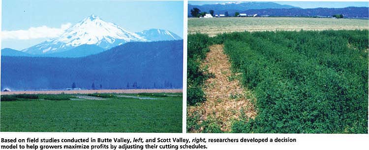
Based on field studies conducted in Butte Valley, left, and Scott Valley, right, researchers developed a decision model to help growers maximize profits by adjusting their cutting schedules.
The price differences between hay quality categories vary widely from year to year due to a number of complex supply and demand factors. The Northern California price differentials ranged from 24.4% to 74.3% over a 10-year period (fig. 1). The decision to cut for quality or yield depends upon the magnitude of this price difference.
Considering how much prices have varied over the past decade, no single strategy was always best. This point is illustrated by the 1996 and 1999 data, which represent extremes in the market price differentials. In 1996, the price differential was only 24.4% between Premium and Fair. Using the decision rule for our intermountain grower results in a decision to cut for yield (Fair quality) on both the first and second cutting (considering Premium-Good and Good-Fair comparisons). On the other hand, in 1999 the wide price differentials lead to decisions to cut earlier for higher quality on both cuttings.
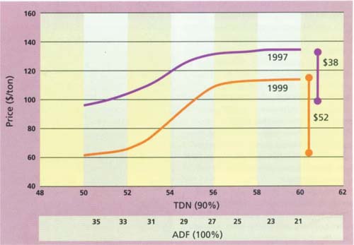
Fig. 3. Idealized relationship between forage quality (ADF, TDN) and alfalfa price ($/ton) for high-price (1997) and low-price (1999) years. ADF is acid detergent fiber (100% dry matter) and TDN is total digestible nutrients (California equation, 90% dry matter).
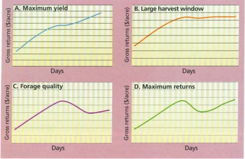
Fig. 4. Four typical outcomes of harvest timing on gross returns, based on field data and hypothetical quality-price relationships. These result from changes in the price difference between higher and lower quality hay under various market conditions. (A) Maximum yield produces the greatest returns; (B) with a large harvest window, yield and quality equalize after a certain point; (C) high forage quality produces the greatest return, then profitability rapidly, declines; and (D) two optimum points of return — quality, followed by yield. Each vertical column represents 1 day.
Idealized price curves
The four categories used by USDA to characterize the alfalfa market contain a range of forage quality values. To analyze potential returns, a continuous sequence of forage quality values along with corresponding prices is needed. We developed idealized price curves for two distinct price years to show the change in price for each incremental change in TDN or ADF (fig. 3). These curves represent a high-price year (1997) with a relatively small Premium-to-Fair price differential and a low-price year (1999) with a large Premium-to-Fair price differential. The curves were based partly on real data from 1997 and 1999, and on discussions with growers and hay brokers about market behavior.
Reflecting the behavior of the California market, there are three distinct segments to the price curves. For TDN values of 56% and above there is very little change in price for each incremental change in TDN. Similarly, there is little drop in price associated with each change in TDN at the low-quality end of the curves. However, at the center portion of the curves, when alfalfa hay goes from 56 to 54 or 53 TDN, there is a precipitous drop in price. This is characteristic of the commonly observed “dairy hay” cutoff perceived by the market. Under current market conditions and perceptions, alfalfa above 55% to 56% TDN (below 27 to 28 ADF) is considered dairy quality, while hay lots below this level of quality are used for dry cows and other nondairy classes of animals.
Timing effects on gross returns
We also calculated gross grower returns within a growth period. The yield (ton/acre), with its corresponding forage quality, was simply multiplied by the associated price from the price curves in fig. 3.
Projections under different price relationships suggest four likely outcomes for gross returns (fig. 4A-D). With all outcomes it was not profitable to cut very early for extremely high-quality alfalfa, greater than about 58 TDN (less than about 24 ADF). The price premiums received never compensated for the lower yields obtained that early in the growth cycle. The first possible outcome (fig. 4A) is where maximum yield always optimizes returns. In this case the price premium obtained for dairy-quality alfalfa is so low that the effect of increasing yield overrides any effect of forage quality on price. This scenario occurs most frequently in high-price years.
The second outcome (fig. 4B) affords a large harvesting window. The drop in price associated with a reduction in forage quality is equally offset by an increase in yield, so returns remain relatively constant after a certain time in the growth cycle.
In the third outcome (fig. 4C), gross returns are maximized by producing alfalfa with high forage quality just at or above the cutoff for dairy-quality alfalfa. The grower must cut for quality and capture the Premium price, or risk loosing profitability. Any increase in yield after that point is insufficient to compensate for the large price drop.
In the last outcome (fig. 4D) there are two potential points of maximum return. Returns peak first when alfalfa is cut for quality. After that point, a slight increase in yield is insufficient to compensate for the large drop in price so returns decline. However, if harvest is delayed long enough there is a significant yield increase that compensates for the price drop from Premium to Good or from Good to Fair. Which of these four outcomes occurs under real conditions depends on both the alfalfa market and growing conditions.
Analysis of intermountain returns
Gross returns were modeled for the first and second growth periods (figs. 5A and 5B, respectively), using actual field data (fig. 2) and the idealized curves for a high-price and low-price year (fig. 3). In the high-price year (1997), there was less price differential between the Premium and Fair hay compared with the low-priced year. For the first cutting {fig. 5A) this curve is similar to that in figure 4B, with a long harvest window. The situation was quite different in the low-price year (1999), which had a large price differential (fig. 5A). Returns were lowest when alfalfa was harvested at a very early growth stage — when yield is low and forage quality extremely high. Returns peaked in the range where alfalfa is generally considered dairy quality. Returns then declined as harvest was delayed, until returns began to increase again when the increase in yield nearly compensated for the decrease in quality. So, in this case, returns were highest in the dairy-quality range or when harvest was delayed much later to obtain maximum yield.

Fig. 5. Gross returns per acre as alfalfa matures for (A) first and (B) second growth period. Reflects yield and quality data from the field, with prices representing high-price (1997) and low-price (1999) year. Each vertical column represents 1 day.
The relationship between day of harvest and returns per acre was different for the second cutting, which is mid-summer in the intermountain region (fig. 5B). As stated previously, yield increases and forage quality decreases at a faster rate for the second cutting than for the first (fig. 2). In the high-price year gross returns were highest at maximum yield {similar to fig. 4A). Only near the cutoff for dairy-quality hay did the increase in revenue even show signs of leveling off. However, after a few days delay in cutting, the gross returns continued to increase rapidly. In contrast, figure 4D most closely resembled the shape of the return curve in the poor-price example (1999). If harvest was delayed long enough, returns were greater at maximum yield than at dairy-quality hay.

No single harvest strategy is best for alfalfa. The decision on when to cut should be based on rates of change in alfalfa yield and quality, and the price differential between dairy and nondairy hay.
While this type of analysis can be revealing, growers must recognize the conditions and assumptions that were used. The market behavior was based on data provided by the USDA Hay Market News; local price data may vary. The analysis assumed current pricing behavior, with a tremendous drop in price from 56 to 54 TDN. This is a description of the market in California and may not be a true reflection of the hay's actual feeding value. There are a number of other quality factors in addition to ADF concentration, including digestibility of the fiber fraction, protein degradability and ash. This analysis also assumed that price is determined solely by forage quality (measured analytically by ADF or TDN). There are certainly other factors, especially for nondairy hay, including the overall physical appearance (color and the presence of weeds or mold) and suitability for export or the horse market.
This analysis also assumed that the increase in alfalfa yield over time is linear. In our data sets this was only true within normal cutting intervals. Eventually, as alfalfa becomes over-mature, the yield increase will level off. In addition, this analysis only examines the revenues from a single cutting. The timing of an individual cutting clearly influences the amount of growing time available for subsequent alfalfa cuttings. Therefore, to fully analyze different cutting management strategies it is necessary to consider the entire production season rather than just individual cuttings. This analysis also does not account for the long-term effect of cutting date on stand persistence and weed encroachment. Nonetheless, an economic analysis of the optimum timing for a single growth period is the first step toward a more complete analysis.
Cutting schedules, profitability
Alfalfa cutting schedules have a large influence on profitability in intermountain regions. There is a fundamental trade-off between yield and quality in alfalfa over a growth period, a biological relationship with large economic implications. During the first growth period, average changes in yield over 2 years of study were 80 pounds per day while ADF content increased 0.33 percentage points per day. Second-cut changes in yield were 112 pounds per day and 0.40% ADF per day. An analysis of gross returns using two distinct market years demonstrated that no single harvest strategy is best for all situations. Whether it is more profitable to aim for high forage quality or maximum yield depends on the rate of change in yield and quality and the price differential between dairy and nondairy hay. Since the price differences due to quality attributes vary significantly from year to year, a grower's cutting strategy should be flexible enough to respond to these market fluctuations.
Proper harvest timing can improve returns for intermountain alfalfa