


All Issues
Use of long-range weather forecasts in crop predictions
Publication Information
California Agriculture 44(2):28-29.
Published March 01, 1990
PDF | Citation | Permissions
Abstract
Uncertainties in weather forecasts still present the greatest problem in making useful crop predictions. Weather variables needed for crop growth models are minimum and maximum temperatures, precipitation, and solar radiation. Each of the three potential sources of long-range forecasts of such variables has deficiencies, but improvements offer some encouragement.
Full text
Farmers, commodities dealers, water managers, and others have long sought to forecast production of major crops through the use of models requiring some sort of weather input. Steady strides have been made recently in developing physiological models of crops such as wheat and rice. Such models should include daily minimum and maximum temperatures, precipitation, and solar radiation. Up to now, these crop models have generally been used with past weather observations or statistical weather generators. This report inquires into whether meteorological forecasts can provide variables accurate enough to provide skillful crop predictions.
Types of weather forecasts
Three general types of medium-and longrange weather forecasts are available: (1) 3-to 10-day forecasts of daily weather made by the same numerical weather models used for the typical 1-and 2-day forecasts seen in newspapers or on television; (2) 90-day weather outlooks generated by the National Weather Service and others based on statistical forecast methods; and (3) the relatively recent 10-and 20-day average forecasts made 5 to 30 days in advance from special runs of the operational weather forecast models. To understand the use of these forecasts in preparing crop models, attention must be given to the kind of the forecast weather variables used in each case and to the overall quality of the forecasts.
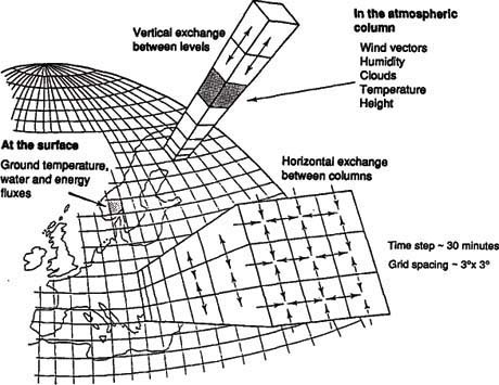
Numerical forecasts. The numerical models are large physical/mathematical computer models of the global atmosphere. These solve six or more coupled equations governing atmospheric behavior for a large number of horizontal and vertical points on the globe. Figure 1 shows the typical grid structure of such models. The spacing between horizontal grids is commonly about 200 km (120 miles). Between 10 and 30 levels are in the vertical columns. Using this system, complicated physical equations can be solved at 150,000 to over 400,000 points around the earth.
These forecasts are begun from observed initial conditions, based on surface, weather balloon, satellite, and various other meteorological observations. Variables are updated in model “time” at intervals of about 30 minutes. The results represent the combined values of weather variables at each of the grids for each 12-hour period in the future. All important weather variables are potentially available, including those necessary for the physiological crop models.
One problem, however, in using numerical forecast variables in crop models is that the model grid spacing of about 120 miles is much larger than the usual agricultural regions of tens of square miles. Moreover, a single model grid may include such diverse surface features as oceans, deserts, and mountains. A question is how one should interpret the average temperature or precipitation for such a large region in terms of the weather actually affecting a crop. Such problems are often overcome by applying model output statistics (MOS). MOS compares large-scale model predictions of temperature or precipitation with observed weather variables for subregions the size of agricultural regions.
An even bigger problem is the uncertainty of weather model forecasts and how they lead to possibly overwhelming uncertainties in crop production forecasts. Figure 2 illustrates a measurement of forecast skill for 500 millibars geopotential height, the most important variable describing largescale air flow, for the model developed at the European Center for Medium-range Weather Forecasting (ECMWF). This model is generally recognized as the best in the world.
The skill is assessed in terms of “anomaly” correlations between the forecast weather minus the model's “climatological mean” and the actual observed weather on the forecast date minus the observed climatological mean. These correlations are very near the maximum value of one for 1-and 2-day forecasts and decrease steadily thereafter. These relatively short-range forecasts have improved since 1972, mainly with the introduction of new computers and finer grid spacing.
The horizontal line on figure 2 is the approximate skill of a persistence forecast, a forecast specifying that the weather tomorrow will be exactly the same as today's. This is generally assumed to be the standard of accuracy that a numerical model must beat to be respectable. At present, this standard is met by the ECMWF forecasts out to 6 or 7 days. The variable geopotential height shown in figure 2 is a measure of the force driving the atmospheric circulation and is the most common measure of forecast skill. Model skills for other variables are generally lower, especially for precipitation, whose forecasts are probably about half as accurate as those shown in figure 2.

Outlooks. The second kind of medium-to long-range forecasts available are statistically derived from models using predictors such as 500 mb geopotential heights, sea surface temperatures, and areas of snow cover. These are made for the United States at the beginning of each 3-month season by the National Weather Service and Jerome Namias, a researcher at the Scripps Institution of Oceanography at the University of California, San Diego. The outlooks are made for average temperature and total precipitation for the contiguous United States on spatial grids like those in figure 1. Outlooks are not forecasts of actual temperature or precipitation, as in the case of numerical models, but are only forecasts of whether the average temperature or precipitation will be above, near, or below the climatological mean. There are thus only three equally likely forecast possibilities.
As with the numerical weather model forecasts, use of outlooks in crop predictions requires estimates of how changes in large-region average temperature and precipitation would affect individual growing areas. Furthermore, estimates of minimum and maximum temperature, rather than mean temperature, and solar radiation would have to be made using statistical analyses of past observations. In addition, seasonal means would have to be translated into typical daily weather. Professor S. Geng at UC Davis has shown that this is possible for monthly mean data using a weather generator, which calculates typical day-to-day weather variations based on past daily statistics for individual weather stations.
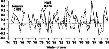
As with the numerical weather forecasts, the largest obstacle to the use of the seasonal outlooks in crop forecasts is the uncertainty in the forecast weather. Figure 3 shows another measure of forecast skill for the precipitation outlooks made by the National Weather Service and J. Namias from 1974 to the present. The skill score in figure 3 is the fraction of grids in the United States with the correct forecast (above, below, or near normal) minus the fraction that is expected to be correct from chance alone, 33%. Both sets of outlooks have both positive and negative skill values. The negative values correspond to forecasts that are poorer than a simple guess. The average skills are positive, but they are quite small. Skill scores for average temperature are similar.
Although these results are discouraging, the outlooks are sometimes accurate and they may eventually be relatively skillful. Although some other long-range weather forecasters might suggest skills much better than those illustrated in figure 3, careful assessment would probably indicate similar results.
Average forecasts. In the last few years, national meteorological centers have begun to experiment with a third type of medium-to long-range weather forecast. The 10-and 20-day average forecasts are done 5 to 30 days in advance and are based on longer runs of the models similar to those used for the 10-day daily forecasts. The skills of the daily forecast decrease rapidly after 10 days, in part because of the nearly chaotic nature of the atmosphere. Nevertheless, it is believed that the skills for multiday averages are likely to be relatively large.
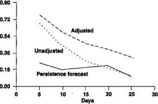
Figure 4 illustrates examples of the skills of such forecasts made by the climate model at the Geophysical Fluid Dynamics Laboratory at Princeton. The anomaly correlations are generally higher for a 10-day average forecast than the daily results shown in figure 2. The correlations also remain higher than those expected from persistence, even for the 25-day forecasts. Furthermore, adjustments of the model predictions, taking into account known model deficiencies, improve the skills considerably. These results are encouraging, because they seem to imply skill considerably greater than those of the statistical/empirical outlooks. As has been true of other numerical model forecasts, the skills of these 10-or 20-day average forecasts seem likely to improve.
Although these average forecasts derived from numerical models seem encouraging, several factors suggest caution in their use. As with all of the forecasts discussed, weather values corresponding to the averages over very large regions must be transformed to values appropriate to the scale of a crop model. Similarly, daily weather variables must be estimated from the 10-or 20-day means. Most importantly, such forecasts have been made for relatively short times. The skill scores in figure 4 thus may be overly optimistic, or perhaps pessimistic.
Conclusions
Before the available weather forecasts can be used in crop production models, a number of technical problems must be overcome. These include the effects of the differences between weather forecast results and crop model requirements in horizontal resolutions, temporal sampling, and specific weather parameters. Most importantly, it is necessary to resolve the question of how to incorporate large uncertainties in any of the long-or medium-range weather forecasts into the crop models.
Even if improvements occur in the future, uncertainties in the forecasts could suggest that crop predictions based only on a single set of forecast variables would be of little value. The known uncertainties will probably require that the crop models be run a number of times with various weather inputs, ranging around the predicted values. In this way, a range of crop predictions will be available whose variations will give a measure of the uncertainties of the prediction.
It will be necessary to assess how best to use the crop predictions. One question, for instance, is whether there are any management decisions likely to be profitable that can be made using a 10-day crop forecast with an average skill of 50%. The ultimate goal must be to maximize the utility of predictions given realistic assessments of their uncertainties.
Use of long-range weather forecasts in crop predictions