The Lake Tahoe Basin is a subalpine ecosystem bordered by the Carson Range to the east (Nevada) and the Sierra Nevada crest to the west (California). This 520-square-mile basin is dominated by the 192-square-mile Lake Tahoe, which is noted for its exceptionally clear water. The lake's water clarity is largely due to nutrient-poor granitic soils in the surrounding watershed and a low watershed-to-lake ratio. Most of the rest of the basin is a nitrogen-poor, mixed-conifer forest ecosystem comprised mainly of fir (red [Abies magnifica] and white [Abies concolor]), pine (lodgepole [Pinus contorta], sugar [Pinus lambertiana] and Jeffrey [Pinus jeffreyi]), and incense cedar (Calocedrus decurrens). Historically, these factors have minimized the flow into the lake of nutrients and sediment that could reduce water clarity.

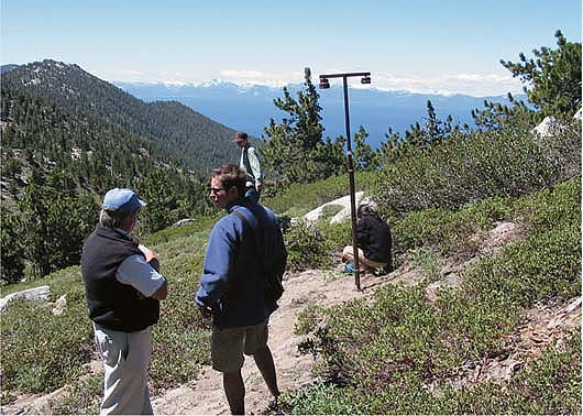
In 2002, scientists constructed passive samplers throughout the Tahoe Basin, including, above, on Diamond Peak, to measure 2-week average ozone and nitric acid concentrations. Air pollutants are believed to be an important contributor to Lake Tahoe's declining clarity.

Since 1967, Lake Tahoe's water quality has declined at an unexpectedly rapid rate, in part due to anthropogenic nutrient and sediment loading (Goldman 1988; Jassby et al. 1999; Murphy and Knopp 2000). The Lake Tahoe Watershed Assessment provided a comprehensive summary of scientific knowledge regarding the factors contributing to the observed water-quality decline and the steps that can be taken to restore the Lake Tahoe Basin ecosystem (Murphy and Knopp 2000). Contributing factors include nitrogen, phosphorus and sediment flow into Lake Tahoe. Murphy and Knopp (2000) reported that atmospheric deposition (gases and particles that enter the lake from the air) accounts for approximately 55% of the nitrogen and 27% of the phosphorus load into the lake. No estimate of atmospheric fine-soil particulate input was presented.

In addition to decreasing water clarity, atmospheric pollutants can affect forest health. It is well established that ambient ozone has pronounced adverse effects on forest health in California's mountain regions (Arbaugh et al. 1998). According to large-scale distribution maps of the Sierra Nevada bioregion, the Lake Tahoe Basin's summer-season, 24-hour ozone levels are 50 parts per billion (ppb) to 60 ppb (Fraczek et al. 2003). Such ozone levels may be phytotoxic (toxic to vegetation) (Krupa et al. 1998) and can adversely affect tree health (Arbaugh et al. 1998). Ozone causes foliar injury (an indicator of tree health) to ponderosa (Pinus ponderosa) and Jeffrey pines in the central Sierra Nevada (Miller et al. 1996), including in the Lake Tahoe Basin (Pedersen 1989).

While there has been extensive water sampling in the basin, air sampling has been limited to two sites at the southern end of the basin, and does not include data on phosphorus or coarse soil particles. Atmospheric deposition could be a major source of nitrogen input and a significant source of both phosphorus and sediment loading, but we lack knowledge regarding the sources and concentrations of these pollutants, the contributions from in-basin versus out-of-basin sources, and the spatial distribution and deposition of atmospheric pollutants. In this paper, we review the air-quality study results that address these questions (NWRA 2004).

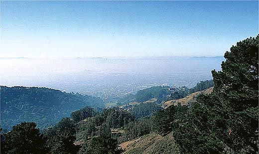
Using atmospheric models, the authors simulated how air pollutants from the Bay Area, above, and Sacramento Valley are affecting the Tahoe Basin. While pollutants are transported from outside the basin, the model suggests that they are significantly diluted by mixing on the western slopes of Sierra Nevada.

Fig. 1. (A) Area of California modeled, with emissions sources (San Francisco Bay Area, Sacramento and Lake Tahoe Basin). (B) In the Lake Tahoe Basin, blue circles designate point sources used to represent mobile and area emission sources. Marked stations are South Lake Tahoe (SOLA), Bliss State Park (BLIS), Thunderbird Lodge (TBLG), Echo Summit (ECHO), U.S. Coast Guard (USCG) and Barker Pass (BARK).

Modeling nitrogen pollution

In terms of hemispheric atmospheric circulations, California is within the latitude range of prevailing westerly winds. However, due to the relatively weak effect of large-scale atmospheric motions, wind patterns tend to be modified by the differential heating between the land and ocean. Previous studies have shown that in California's typical summer wind-flow pattern, marine air penetrates through the Carquinez Strait (in the northeastern San Francisco Bay) and bifurcates around the Bay's Delta region into south and north branches (Moore et al. 1987; Zaremba and Carroll 1999). This primary pattern is superimposed by thermally driven daytime upslope and nighttime downslope flows, making pollutant transport eastward possible from heavily polluted regions, such as the San Francisco Bay Area and the Sacramento Valley, up into the Sierra Nevada.

In order to quantify how much nitrogen these winds bring into the Tahoe Basin, we used the advanced numerical atmospheric models CALMET/CALPUFF (Scire et al. 2000) and MM5 (Grell et al. 1995) to estimate the contributions from both in-basin (such as cars and trucks) and out-of-basin (such as industry, cars and trucks) nitrogen sources. The area we modeled was selected to simulate how the basin's air is affected by pollutant transport from the Sacramento Valley and San Francisco Bay Area (fig. 1A).

In this study, the comprehensive CALMET/CALPUFF air-quality modeling system was coupled with a numerical weather model called MM5. The output from the MM5 model was coupled with available surface and upper-air meteorological measurements to enhance the accuracy of the predictions (fig. 1B). The CALMET/CALPUFF simulation grid (fig. 1A) contained 250-by-265 cells, each 1 square kilometer (0.61 square miles), and the lower left grid corner was referenced at 37.10° N and 122.70° W.

In order to accurately predict regional versus local transport and dispersion, information on pollutant (such as oxides of nitrogen) emission rates was critical. This data was obtained from the California Air Resources Board (CARB). For the Lake Tahoe Basin, we prepared hourly emission allocations based on the CARB inventory. Hourly emissions from Truckee, Reno, Interstate 395 and the west Sierra foothills were also included. Sensitivity studies were performed for the model calibration.

One of the key pollutants leading to nitrogen deposition into the lake is nitric acid (HNO₃). This pollutant is not directly emitted from sources but is formed through a series of atmospheric reactions involving oxides of nitrogen and hydrocarbons. Estimates of nitric acid formation and atmospheric concentrations were made using the previously described modeling system.

Simulations were performed for three selected cases coinciding with previous nitric acid measurements during summer 2000 (Tarnay et al. 2001, (2005). These cases were selected based on a range of wind patterns and high/low ambient nitric acid. Analysis of surface observations (surface wind frequencies and precipitation) and large-scale synoptic pressure systems (500 millibar wind and pressure maps) showed that the selected cases were climatologically representative of summer 2000. MM5 simulations were performed with two-way nesting for a 4-day period. The spin-up time was 12 hours. In order to model regional-scale transport and reduce the effect of boundary conditions, the CALMET/CALPUFF modeling system was run for 72 hours for each of the selected cases.

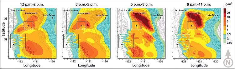
Fig. 2. Evolution of nitric acid (μg/m³) plume from California's Central Valley, Aug. 28, 2000. Concentrations (filled contours overlaid with topography) are averaged over 3-hour intervals. The enclosed areas surrounding Sacramento and San Francisco regions designate the emission sources. Note the effects of daytime upslope flows and nighttime downslope flows; pollutant concentrations at elevated regions are low, implying minimal nitric acid transport to the Lake Tahoe Basin.

Airborne plume mostly diluted

The overall simulation results indicated that there is pollutant transport from the Sacramento Valley and San Francisco Bay Area to the Lake Tahoe Basin (fig. 2). However, these pollutant concentrations were significantly diluted by mixing with other air masses on the west slopes of the Sierra Nevada at increasing elevations, as measured in previous studies (Carroll and Dixon 2002; Dillon et al. 2002; Bytnerowicz et al. 2002). While part of the emissions plume can progress over the Sierra Nevada to the Lake Tahoe Basin, nitric-acid ambient air concentrations are extremely low. In addition, later in the day, downslope winds carry the plume back to the Central Valley. (Simulations of in-basin and out-of-basin emissions were performed separately in order to determine their relative contributions; the impact from in-basin emissions is not shown in figure 2.)

On the other hand, the results also showed that the predicted nitric acid concentrations due to local sources were in good agreement with actual measurements. For example, 90% of the predicted nitric acid concentrations were due to local sources, and the predicted concentrations comprised 65% of the average measured values (Tarnay et al. 2001) in all the monitoring locations around Lake Tahoe. Emissions of nitrogen oxides from other nearby source regions such as Reno and Interstate 80 were two to three orders of magnitude smaller than those from the San Francisco Bay Area and the Sacramento Valley, and had no significant predicted impact.

In short, while the results of this work suggest that daytime pollutant transport from upwind of the Lake Tahoe Basin appears to be likely, the amount of nitric acid transported from outside of the basin is much less than that from in-basin sources. In order to better quantify these contributions, additional study is needed on long-term transport effects under different meteorological patterns that could lead to increased transport to the basin.

Measuring ozone and nitric acid

On-ground monitoring of pollutant concentrations helps to test the results of the modeled air-pollution distribution predictions. One of the great difficulties in evaluating the transport of air pollutants into the Tahoe basin is the lack of monitoring data on the upwind western slope of the Sierra Nevada. We were able to address this problem by using inexpensive passive samplers, which allowed us to deploy a monitoring network of unprecedented scope throughout the region. To provide measurements in support of the meteorological modeling described in the previous sections, we studied two pollutants: ozone (O₃), long known to transport into the basin, and nitric acid. We selected 32 monitoring sites to assess air pollution levels in and around the Lake Tahoe Basin. The sites were selected in open terrain located on a western aspect, with free air movement from all directions. The passive samplers measured 2-week average ozone and nitric acid concentrations throughout the 2002 smog season.

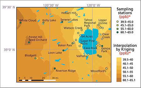
Fig. 3. Seasonal average distribution of ambient ozone concentrations (ppb)^* in the Lake Tahoe Basin and its vicinity, summer 2002. Shaded areas represent concentrations determined by interpolation of the observed data by Kriging. Maximum levels of ozone were observed to the west of the lake, but are not transported to the basin.

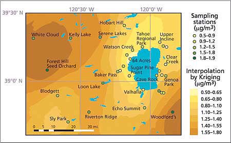
Fig. 4. Seasonal average distribution of ambient nitric acid concentrations (μg/m³) in the Lake Tahoe Basin and its vicinity, summer 2002. Maximum levels were observed west of the Sierra Nevada crest and lowest levels are near the west shore of the lake.

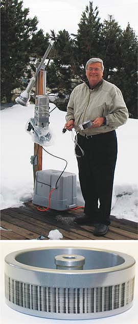
Top, UC Davis professor Tom Cahill sets up a DRUM sampler at South Lake Tahoe. Bottom, the sampler shows the pattern of very fine, phosphorus-rich aerosols collected over a 3-week period. The dark bands occur in the morning and evening, when the wind stagnates.

Pollutant distribution maps were developed with geostatistical software (ARC/INFO Geostatistical Analyst; ESRI, Redlands, Calif.) that uses values measured at sample points at different locations in the landscape and interpolates them into a continuous surface. Using a set of measurements in a given study area, a spatial model of ozone concentration was constructed (Fraczek et al. 2003). Techniques were then used to develop prediction maps of the air pollutant's distribution for each individual 2-week sampling period and for the entire season.

The highest 2-week and whole-season average ozone and nitric acid concentrations occurred in the Sacramento foothills, west of the Lake Tahoe Basin. Concentrations of these pollutants were much lower near the lake, especially near the west shore. It appears that the mountain range west of the Lake Tahoe Basin (Desolation Wilderness) impedes the westerly flow of low-layer polluted air masses from the Sacramento metropolitan area and the Sierra Nevada foothills, limiting pollutant transport into the basin. East of the lake, ozone and nitric acid levels generally increased with distance from the South Lake Tahoe community urban area.

Over the course of smog season, there was a clear pattern in ozone and nitric acid concentrations. For the entire study area, the lowest levels occurred during the first halves of July and October, and the highest levels occurred during the second half of August (figs. 3 and 4). The highest levels of ozone and nitric acid in August coincide with traffic-related high emissions of nitrogen oxides and volatile organic compounds (VOC), high temperatures and solar radiation — all factors promoting the generation of these photochemically produced air pollutants.

Foliar injury rates low

To estimate the effects of elevated ozone on forest health, we reviewed the results of studies conducted by the USDA Forest Service in the 1970s. USDA scientists conducted studies to evaluate foliar injury, applying the Ozone Injury Index (OII) methodology, in the Sierra Nevada and the San Bernardino mountains (Miller et al. 1996). Foliar ozone injury was evaluated at 25 preexisting study sites in the Lake Tahoe Basin. The sites were originally established in the late 1970s to each contain 15 mature ponderosa pine trees, but as few as six of the original trees remained at some of the locations by the time of the foliar-injury evaluation study.

Overall, 23% of the trees evaluated had foliar ozone injury but the average OII was only 17.3 (100 indicates the highest level of injury), which shows that the injury occurring to the pines in this area is slight. In addition, no discernible spatial patterns of injury were observed between sites, so the degree of ozone injury likely depends on micro-site growing conditions as well as on the genotypic and phenotypic responses of individual trees to ozone air pollution.

Fig. 5. Size-segregated phosphorus measurements (μg/m³) in 2002 for (A) winter (eight particulate size fractions) and (B) summer (four fine particulate size fractions to better show smoke and exhaust). The maximum levels of phosphorus were observed in the largest size fractions, winter and summer, indicating that resuspended geological material was the major pollutant source.

Measuring phosphorus

Phosphorus, which comes into the lake from both sediment in stream runoff and airborne particles, is presently the limiting nutrient for algal growth, a major factor in the lake's clarity decline; while all pollutants entering Lake Tahoe must be reduced, nitrogen pollution is currently so high that the most effective strategy for the time being is to reduce phosphorus. About one-fourth of all phosphorus comes from the air, as shown by the phosphorus data from deposition buckets on and near the lake, but phosphorus is rarely seen in the existing ambient air samples. One possibility is that phosphorus occurs in particles larger than those collected by current in-basin, filter-based air samplers, which only measure fine particles below 2.5 microns (μm) in diameter.

In order to assess the airborne sources of phosphorus, measurements were performed in January and August 2002 using a particulate sampler developed at UC Davis (Cahill and Wakabayashi 1993). In contrast to filter-based measurements, this sampler allowed for measuring particles in eight size-segregated fractions, ranging from 35 μm (roughly a high-volume [Hi-Vol] inlet to catch coarse soil aerosols) to 0.09 μm (to catch diesel and smoking car exhaust). In addition, the UC Davis participate sampler allowed for better source identification because it has a high time resolution (3 hours). Finally, this sampler resulted in an order of magnitude better detection of phosphorus than the filters (Bench et al. 2002) because elemental analysis for phosphorus was performed by synchrotron X-ray fluorescence (S-XRF). Samples were collected at the South Lake Tahoe site for 12 weeks in winter and 6 weeks in summer to allow analysis of synoptic weather patterns.

TABLE 1. Sources and estimated tonnage of phosphorus deposition in the Lake Tahoe Basin

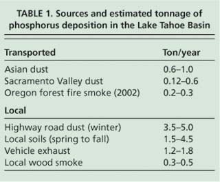
Most of the phosphorus observed during the winter and summer occurred between the 2.5 and 35 μm size fractions, consistent with the sources being resuspended road dust and soil (fig. 5). Previous studies in the area used samplers with a 2.5-μm upper cut-point and would have missed this contribution. This implies that most of the phosphorus comes from in-basin sources, since particles in this range tend to deposit rapidly and so are rarely transported far in the atmosphere. We can estimate the phosphorus deposition from a range of sources based on these particulate sampler data and earlier data using the Lake Tahoe Airshed Model (LTAM) (Cahill and Cliff 2000) and estimated deposition velocities (Seinfeld and Pandis 1998) (table 1).

While these results are highly uncertain, especially because they are based on a single, near-roadway South Lake Tahoe site, together they imply that the majority of phosphorus deposition in the Tahoe Basin can be attributed to local sources from roadway sanding and salting in winter, local soils in summer and vehicle exhaust. Furthermore, some of the out-of-basin sources may not occur routinely. The 2002 Oregon forest fires were unusually severe, and showed a high phosphorus content not seen in less violent fires such as prescribed burns (Turn et al. 1997). The Asian dust values in particular are uncertain and highly variable from year to year, depending on the strength of the dust storms in Asia and the location of the Pacific high-pressure system and winds, which can push Asian dust north into Canada and cut off transport to California, as happened in 2003. It should also be noted that these measurements represent total phosphorus, as opposed to bioavailable phosphorus, and thus have uncertain impacts on algal growth.

Sources of Tahoe air pollutants

Taken together, our review of several important studies indicates that out-of-basin sources are not the major contributors to the observed levels of air pollutants in the Lake Tahoe Basin. For example, the advanced numerical modeling approach found that 90% of predicted nitric acid in the basin came from precursors emitted within the basin. The models attributed the minimal contribution from out-of-basin sources to a number of factors, including dilution, dispersion and minimal pollutant flow into the basin. Similar conclusions were reached by the studies investigating forest health and the sources of phosphorus in the Lake Tahoe Basin. Based on these findings, the most effective strategy to reduce the impact of atmospheric deposition on the lake's clarity and in-basin forest health would be to control local pollutant emissions.

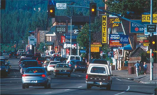
Out-of-basin pollutants are not the major contributors to air pollution in the Tahoe Basin; rather, local sources are having the most significant effects on air and water quality, and forest health. Above, Highway 50 in South Lake Tahoe.