


All Issues
Income risk varies with what you grow, where you grow it
Publication Information
California Agriculture 46(5):14-16.
Published September 01, 1992
PDF | Citation | Permissions
Abstract
Farmers seeking credit today are up against a lending “crunch” that is forcing them to re-assess what they grow and where they grow it. To assist those looking for new market opportunities, a new study offers ways of calculating the kinds of financial risks that concern the lenders who read today's credit applications.
Full text
Despite declining interest rates, many farmers and ranchers are having difficulty obtaining business loans because a credit “crunch” is running its course in agriculture. In this new credit environment, lenders no longer view borrowers as just “farmers”; rather, they are seen as producers of specific enterprises that vary in profitability.
This study offers to explain the change in lenders' views and the implications for California's agricultural sector, and to provide information about the kinds of calculations farmers need to make in assessing market opportunities. Estimates of income variability for a cross-section of crops are presented in an index farmers can use when deciding on what to produce. The simple format enables the user to make choices based on the financial risk involved in raising a particular crop — the major concern of lenders — and to include the information on credit applications.
Today's credit environment
Banks are tightening credit standards. The farm financial crisis of the mid-1980s and the Savings and Loan crisis have shown lenders the risks of holding predominantly real estate loans. The result has been a shift from the common practice of lending on equity to lending on income. Lenders no longer want to foreclose on property and take their chances selling in real estate markets that may decline rather than rise as they did in the past. However, money is still available to agriculture.
“There is no credit gap for creditworthy borrowers,” Michael Grove told the House Subcommittee on Conservation, Credit, and Rural Development. The chairman of the American Bankers Association's Agricultural Bankers Division defined a credit-worthy borrower as one “who has the ability to service debt, based on past performance and projected future profitability.” The “ability to service debt” means that a borrower pays all debts in a timely manner from gross income generated. This illustrates that credit analysis has shifted from the borrower's balance sheet to the income and cash-flow statements.
In California, this shift has led to emphasis on the business risks faced by agricultural producers, including (1) production and yield risks, (2) market and price risks, and (3) income risks. Production risks are largely beyond the control of a producer. Market and income risks, however, are controllable to some extent. Thus, lenders want borrowers to account for the risk/return tradeoff involved in assessing markets.
In particular, lenders are paying more attention to the volatility in incomes of certain crops, rather than expected farm income levels. Crops vary in degrees of production and price risk. Also, geographic regions for a single crop vary in profitability. Therefore, different levels of income risk can be expected. Lenders are beginning to incorporate these differences into credit evaluations.
Lenders will (and borrowers must) consider both absolute risks and relative risks in specific enterprises. A method of doing this is presented below; the first step is measuring financial risk.
Financial risk
In this study risk is defined as volatility or fluctuation. Traditional measures of risk are based upon the standard deviation (SD) of historical price and net income data for individual crops. Combining SD with mean (average) net income data over a time period enables a new absolute measure, probability of loss (PL), to be calculated for a product's market. This measure indicates the chance (in percentage terms) that an average producer in a particular county will generate a negative annual net income from a specific product.
The PL is found by calculating a “z” score and finding the relevant probability for that z value in a statistical table. The z is calculated as
z = E(Ri)-k/si (1)where E(Ri) = the expected (average) return or income from enterprise i, k = some critical value, and σi = the standard deviation of income from enterprise i.
The value of k is usually made zero, but it can be made some other critical level of income. The PL is the chance of earning an income below k. By making k = 0, the PL is the chance of suffering a loss. If some other value is used for k, such as the amount of income needed to cover the payments on a new loan under consideration, the PL found represents the probability of earning insufficient income to cover k; in other words, the PL would indicate the chance of defaulting on the loan.
The calculated z score is looked up in a statistical table for the relevant distribution of incomes to get the PL estimate. For example, most of the time it is reasonable to assume that incomes are normally distributed; therefore, table 1 can be used. If a z of 1.15 were calculated (using k = 0), the normally distributed values in table 1 indicate that there would be a 12.51% (about one out of eight) chance of a negative income occurring for the enterprise.
As noted, the PL is an absolute measure of income risk for an enterprise in a specific market. However, this measure facilitates a comparison of relative risks between crops and locations that is shown below with empirical examples from California markets.
Data used in this study include annual observations reported by county for each product. Values are averages for yield per acre and price per ton. The data were collected by county Cooperative Extension staff of the University of California. For most products the period 1958–86 is covered. Because nominal prices include the influence of inflation, the series was adjusted into “real” terms using the index of farm prices received. The index used is that reported in the Economic Report of the President, 1988, adjusted so that 1986 = 100.
Production and price data are combined with average cost data for each product to generate estimates of income. Gross revenue per acre is calculated by multiplying price (P) times yield (Y). Costs per acre (C), as reported in Extension budgets published for each crop by county, include total fixed and variable costs of production. Therefore, for each crop i average net income per acre at time t is
Rit = [(PY)-C]it (2)Absolute risk
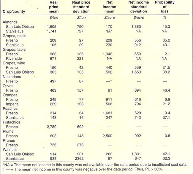
In table 2 and table 3, price and net income data are summarized for a cross-section of field crops and tree and vine crops, respectively, to illustrate the absolute risk in producing each enterprise. For most crops, data from two counties are presented to demonstrate the variability in results across locations. The PL values reported were calculated using k = 0.
Interpretation of PL results in the last columns of table 2 and table 3 is straightforward. The values presented are the probabilities of suffering a loss for specific enterprises listed. For example, Fresno County alfalfa hay producers have a 33.4% (one out of three) chance of losing money in any particular year, according to historical data. If the year being forecast is expected to be typical of years in the data set, PL results are good measures of income risk. Unusual circumstances, like a drought, may raise the level of income risk (the PL), but the absolute amount of increase is not predictable.
Another aspect of the results, which comes from using historical data and a statistical table to find the PL, is that PL values will range between 0 and 100%, but will never be either 0 or 100%. Although some crops have low PL values, such as the 0.5% for carrots in Monterey County, none will have a zero value. This is a characteristic of statistical tables for distributions, but in this application it reminds us that there is always some chance of suffering a loss in agricultural production.
On the other end of the distribution, a grower should not consider any crop with a PL of 50% or greater unless the grower expects better-than-average results. A PL value of 50% indicates that average income over the data period was zero; thus, on average, growers in that county made no money over the period. Even though above-average growers were making money, such a high PL indicates that risks incurred may not be justified by income level. Nectarines in Fresno County may be an example of such an enterprise (table 3). On the other hand, pistachio results for Fresno County may be misleading. The fact that pistachio production was being established during the historical data period may have biased results downward. In this case, only recent farm-level data should be used to calculate the PL.
Relative risk
Lenders are diversified across products and locations, so they are concerned with relative risks, as well as absolute risks, in lending to a particular grower. The PL measure can also be used to assign a relative risk rating to each product market. In general, the method is to rank a product in two ways: (1) A product's risk is ranked according to its PL relative to the entire list of crops grown in the county, and (2) all production regions for a single enterprise are ranked according to their PLs.
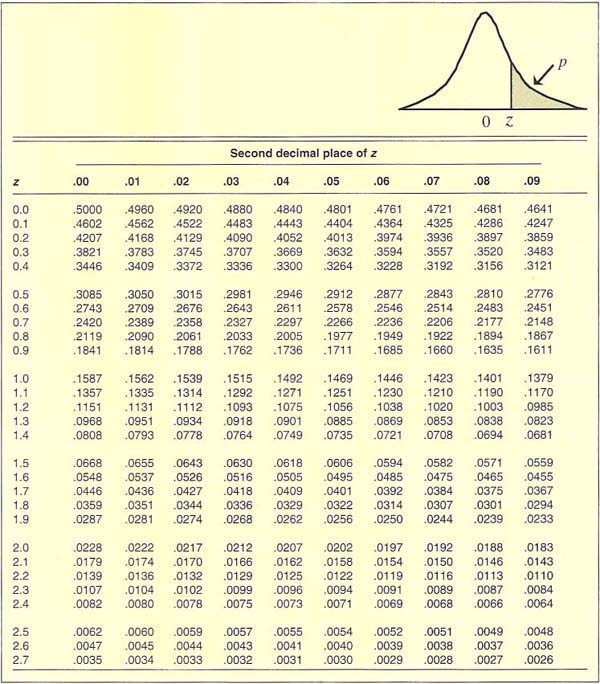
TABLE 1. Normal distribution. The tabled entries represent the proportion p of area under the normal curve above the indicated values of z (example: .0694 or 6.94% of the area is above z = 1.48). For negative values of z, the tabled entries represent the area less than z (example: .3015 or 30.15% of the area is beneath z = −.52)
Ranking enterprises within a county relative to their PL is a means of rating the riskiness of the grower's chosen enterprise versus the alternatives available. For a lender, this is a way to identify the lowest-risk borrowers in a region. For example, table 2 and table 3 list a number of crops grown in Fresno County with peaches ranked best in terms of PL. This means that lenders concerned only with the risk of default will favor peach producers over other potential borrowers in the county. This could mean producers of other crops will have more difficulty in gaining loans or they may have to pay a higher interest rate than peach producers to compensate the lenders for accepting the higher risk.
Peach producers in other counties may not fare as well. Table 3 indicates that Stanislaus County peach growers face greater risks than do Fresno County peach growers. It is most likely that a lender deciding between potential borrowers in the two counties would choose to lend to Fresno growers first, based on their PLs (0.4 versus 37.1%). This also helps explain differences in credit availability and interest rates across locations.
Implications of credit crunch
The credit crunch is affecting many agricultural producers in California. Some have not been able to borrow the amounts they want, and interest rates have become higher for some growers than for others. Even though interest rates have trended downward for some time, rates have not fallen equally for all enterprises due to perceived differences in risk among products. The drought and the freeze have caused many lenders to re-assess the risks involved in production across products and locations.

Although no lenders have completely withdrawn from the agricultural sector, large diversified lenders have tightened loan requirements, causing some borrowers to be dropped as customers. Some lenders are re-evaluating their minimum levels of risk-return tradeoff for loans. This means that those producers that large diversified lenders consider risky will have to seek capital elsewhere with their best prospects being small, local lenders. This situation creates the danger that over time small rural lenders will accumulate much riskier loan portfolios than large lenders, making the rural banks more likely to fail if they suffer loan defaults. To avoid such risk, rural lenders may have to turn borrowers away, and some agricultural producers will be without sufficient capital to operate effectively.
To deal with tighter credit, individual growers may need to adjust cropping plans. In Fresno County, for example, crops usually considered safe (because there is always a market for them or because potential losses will be smaller), such as alfalfa hay and field corn, are shown in the analysis here not to be as safe as some crops commonly considered “risky,” lettuce for one. As shown in table 2, the risk/return tradeoff in lettuce gives it a better PL, 14.5%, than for hay and corn (33.4% and 30.2%, respectively). Thus, Fresno growers with land suitable for lettuce could increase their profits and lower their risk of loss by shifting from hay and corn into lettuce. For the same reasons, lettuce growers in Monterey County may be better off shifting from lettuce to carrots.
When making investment decisions, both lenders and borrowers have always studied income levels, adjusted by risk. Lenders, however, have traditionally weighted risk much higher in the decision process than have agricultural borrowers. Lenders have a shorter investment horizon than borrowers and, hence, are less willing to risk loss (loan default). What the current credit crunch indicates is that lenders are placing even greater weight on the risk factor in assessing the risk/return tradeoff. This shift in credit requirements increases competition among producers across crops and locations when a diversified lender is deciding to whom it will extend credit. Although such competition improves efficiency in statewide resource allocations over time, it also creates some dislocation in cropping patterns and in the structure of resource allocation among market participants.
Clearly, this situation affects everyone in agriculture. Clearly, also, individual producers need to respond by incorporating the use of a risk analysis tool, such as the PL measure, in choosing enterprises.
Income risk varies with what you grow, where you grow it