


All Issues
Microcomputer program ACRE helps answer: When water is limited, how many acres do you plant?
Publication Information
California Agriculture 46(3):7-9.
Published May 01, 1992
PDF | Citation | Permissions
Abstract
A microcomputer program, ACRE, calculates the number of acres of field and row crops to plant, given a limited water supply. Inputs include crop water balance parameters and the anticipated supply of irrigation water. This program is useful for determining how many acres to plant when the goal is to avoid the kind of water stress that impairs marketable production of a crop.
Full text

Drought-stressed corn showing curled leaf response.
Insufficient water supplies can decimate an irrigated crop. As water becomes scarce, the first management step is to evaluate and improve the irrigation system to attain maximum application efficiency and avoid deficit irrigating. Application efficiency (AE) is the ratio of applied water (AW) stored in the crop root zone to the total water applied. Reducing surface runoff and distributing water more evenly improves AE and decreases the total depth of AW per acre needed to refill the soil. Water can then be distributed over more acres.
Irrigation regimes
Full irrigation. The terms full irrigation and deficit irrigation refer to irrigation applications where the goals, respectively, are to refill and not to refill the crop root zone to field capacity. The ACRE program assumes full irrigation when determining acres to plant. When full irrigation is employed, applied water (AW) is predetermined, using soil water depletion (Dw) before irrigation and application efficiency (AE) from previous system evaluations as:
AW = DW-AE (1)where AW and Dw are in inches and AE is expressed as a fraction. Calculating AW with Eq. 1 ensures that (a) the mean depth of water infiltrating the low quarter equals Dw and (b) soil water content returns to near field capacity in 87.5% of the field. The low quarter is that quarter (25%) of the field infiltrating the least water. When applications are properly timed and full irrigation is employed, crop water stress is minimized and the crop normally accumulates the maximum (potential) seasonal evapotranspiration (PMET).
Good irrigation scheduling is important to acreage planning; its goal is to determine when and how much water to apply for optimal production. For most crops, marketable production is optimized by supplying sufficient water to avoid plant water stress. Exceptions include cotton, sugar beets and processing tomatoes. Recent work by D. W. Grimes, water scientist at UC’s Kearney Agricultural Center, shows optimal cotton production occurs when moderate water stress reduces seasonal crop evapotranspiration (ETs) less than PET. Similarly, there is evidence that moderate water stress during late season increases the sugar content of sugar beets and increases soluble solids in processing tomatoes. In these three crops — cotton, sugar beets and tomatoes — moderate water stress improves product quality and growers often get higher prices.
Planning the number of acres to plant involves careful assessment of irrigation scheduling using a water balance procedure. Irrigations are timed to avoid stress or to achieve a specific level of plant water stress. Soil water is depleted by evapotranspiration and is replaced mainly by irrigation. However, sources of water, in addition to irrigation, include contributions from (1) stored soil water, (2) effective rainfall, (3) shallow water tables and (4) plant interception of fog. In many cases, ignoring these other sources of water leads to inaccurate scheduling and overirrigation.
Water stored in the soil from the previous season or from off-season rainfall can contribute to crop water use. The amount supplied equals the difference between the preseason and end-of-season soil water contents. The difference is referred to as preseason usable water in the ACRE program. For efficient irrigation planning, preseason soil water content should be measured and a desired end-of-season soil water content identified to calculate preseason usable water.
Rainfall contributions (effective rainfall) can be a significant source of water for evapotranspiration of winter crops in California. Discussing methods to estimate effective rainfall is beyond the scope of this article. Simply stated, effective rainfall is the portion of rainfall that is stored in the crop root zone or coats the plants during the cropping season.
Contributions from shallow water tables are site-specific, depending on water table depth, crop rooting, soil characteristics and water quality. Water table contributions to crop water needs can be large, and ignoring them can lead to significant errors in irrigation scheduling.
Plant interception of fog by crops grown in coastal areas and interception by winter cereals can be appreciable. Water gained by plant interception of fog has been observed to contribute more water to a crop than is lost on some days. Evaporation of intercepted fog reduces the energy available for transpiration and, therefore, soil water extraction. Dw is overestimated in foggy areas when interception is not considered.
Deficit irrigation. In deficit irrigation, the depth of water infiltrated into the low quarter is less than Dw. This leads to a decline in mean soil water content and an increase in spatial variability of soil water content throughout the field. Declining soil water content can cause water stress, reduced ETS and lower yield. However, spatial variability of water stress makes it difficult to estimate the effects of deficit irrigation on crop yield.
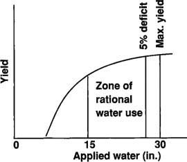
Fig. 1. Relationship between absolute yield of cotton and applied water, showing a zone of rational water use.
Yield predictions are often based on correlations between yield and ETs rather than on deterministic relationships between yield and quantifiable plant water stress. This in itself presents a problem when employing deficit irrigation to stretch limited water supplies over more acreage. Furthermore, uneven application of irrigation water complicates the use of production functions for planning acres to plant. In full irrigation, applied water is determined using Eq. 1 to ensure that 87.5% of the field receives a depth of water exceeding Dw. When a crop is deficit irrigated, less water is applied and the percentage declines. Portions of the field receiving a depth equal to or greater than Dw are expected to attain maximum production, and the deficit irrigated parts may exhibit yield reductions. Because of this spatial variability, deficit irrigating results in a curvilinear relationship between yield and applied water (AW).

The previously mentioned Grimes research identified the relationship in Figure 1 to show that a rational range of AW exhibits little loss in cotton productivity. This relationship results from uneven deficit irrigation application that leads to spatial variability of water stress. Water stress can reduce absolute yield and ETs, but many interacting physical and biological factors determine the level of water stress. Some of these factors include: (1) crop ability to avoid water stress, (2) crop ability to tolerate water stress, (3) spatial variability in soil water content, (4) soil fertility, (5) crop root distribution, (6) water tables, (7) evaporative demand, (8) irrigation frequency, (9) irrigation distribution uniformity, (10) irrigation water quality and (11) pests. Clearly, predicting yield is complex.
During extreme drought conditions, deficit irrigation may be employed to further stretch water supplies. The influence on yield may be small for deep-rooted, drought-tolerant crops grown on soils with high water-holding capacity; however, deficit irrigation is not recommended for most high-value, fresh market fruit and vegetable crops.
ACRE program’s purpose
The ACRE program simplifies and organizes procedures to estimate the number of acres to plant, based on irrigation water supply. Necessary input variables include seasonal crop evapotranspiration (ETs), application efficiency (AE) and water supply. Possible additional input variables include usable preseason stored soil water, effective rainfall, water table contributions and/or fog interception. In some cases, these additional input variables can be overlooked; however, in other cases, ignoring them leads to serious miscalculations of irrigation water needs. Assuming the mean depth of water applied to the low quarter is equal to Dw, the ACRE program accounts for all possible water sources to more accurately assess irrigation water needs.
Water balance calculations
The amount of acreage to plant depends on a balance between the quantity of water supplied from all sources and expected water losses from the irrigated field. Sources of water include:
Preseason usable water (Uc) Water table contribution (Tc) Fog contribution (Fc) Rainfall contribution (Rc) Applied water (AW)Losses of water from an irrigated field include:
Crop water requirement (ETs Application losses (A1)where crop water requirement is the seasonal cumulative crop evapotranspiration that results in the highest marketable yield. Application losses are calculated from Dw and AE from a previous irrigation system evaluation as:
A1 = AW-Dw = (Dw ÷ AE) − Dw (2)The total of all water sources must equal the total of all losses. Rearranging terms, the AW requirement is calculated as:
AW = (ETs + A1) − (Uc + Tc + Fc + Rc) (3)where all the variables are entered in inches. For example, given the following data:
Variable Inches ETs = 27.0 Uc = 4.0 Tc = 0.0 Fc = 0.0 Rc = 1.0depletion of soil water to be replaced by irrigation is:
Dw = 27.0 − (4.0 + 0 + 0 + 1.0) = 22.0application losses, assuming an AE of 0.8, are:
A1 = (22.0 ÷ 0.8) − 22.0 = 5.5and AW needed for the season is:
AW = (27.0 + 5.5) − (4.0 + 0 + 0 + 1.0) = 27.5 inchesSources of information on how to estimate water supplied by preseason usable water, water tables, fog interception and rainfall are included in the user’s guide for the ACRE program.
Acres to plant
Deciding on how many acres to plant depends on the AW needed for production and the quantity of irrigation water supplied during a season. Water quantities are typically expressed in acre-feet, so the depth of applied water in inches is first divided by 12 to convert to acre-feet per acre. For example, 27.5 inches of water equals 27.5 ÷ 12 = 2.29 acre-feet per acre. Acreage to plant is calculated as the acre-feet of water supplied divided by the acre-feet per acre of AW needed to produce the crop. In our example, if 1,000 acre-feet of water are supplied by a water district and/or pumping ground water, acres to plant are calculated as:
Acres to plant = 1,000 ÷ 2.29 = 437Acreage planning with ACRE
ACRE, a user-friendly program, displays a single screen for data entry and output. Sources of water, the crop water requirement, AE and water supplied for irrigation can be entered and/or edited on the computer screen. A value of zero can be entered for sources of water that are insignificant or unknown. However, ignoring significant sources of water can lead to overestimating water needs and underestimating acres to plant. AE is used to calculate application losses from the water balance. An example of the output using the sample data presented earlier is shown in Figure 2. Using these data, 437 acres should be planted.
Microcomputer program ACRE helps answer: When water is limited, how many acres do you plant?