


All Issues
Economics of agricultural drainage policies
Publication Information
California Agriculture 44(4):8-10.
Published July 01, 1990
PDF | Citation | Permissions
Abstract
Policies to reduce agricultural drainwater in the San Joaquin Valley are complicated by different existing drainage conditions on farms. Drainwater reduction policies that address such variations will be more efficient in achieving regional drainage goals.
Full text
The California State Water Resources Control Board has adopted water quality guidelines for the San Joaquin River that include maximum concentrations for selenium, boron, and molybdenum. One source of these elements is agricultural drainwater. The Board suggests that a selenium standard of 5μg per liter can be achieved by reducing drainwater by 30% in a 94,000-acre problem area. Irrigation and drainage districts in the region are implementing plans to reduce the volume of drainwater leaving their boundaries.
The drainwater collected in these districts, which range in size from 10,000 to 60,000 acres, may result from both point source and nonpoint source contributions. Deep percolation on a field without a drainage system may contribute to a high water table that is drained by systems installed on neighboring farms. Drainwater collected in one drainage system may thus have been generated by other farms in the area. Determining the amount of drainwater actually produced by an individual farmer may be difficult and prohibitively expensive.
Regional and district-level drainwater policies must address nonpoint source contributions if drainwater is to be reduced without undue costs. The economic impact of district-level drainage policies will vary among farms with different drainage conditions, since for some farmers it will be easier to reduce drainwater levels than for others. Policies that appear to be equitable may actually cause disproportionate reductions in farm-level income.
We have used an optimization model based on crop production, irrigation, and drainage data collected in the Broadview Water District to examine the economic impacts of selected district-level drainage policies. Our goals were to examine the extent of nonpoint source contributions to the drainwater collected in Broadview, to estimate field-level drainwater and crop yield equations, and to include this information in a district-level drainage policy model.
Data
Irrigation and drainage data collected in the Broadview Water District describe significant variation in the volume and quality of drainwater collected by a set of 25 subsurface drainage systems that service 6,500 of the district's 9,500 acres. Most of the systems were installed in the late 1960s and mid 1970s at spacings that range from 50 to 500 feet and depths that range from 6 to 9 feet. The average salt concentration in biweekly drainwater samples during the 1988 crop year ranged from 4.9 decisiemens per meter (dS/m) for one drainage system to 11.0 dS/m for another. The mean of all system averages in the district was 8.1 dS/m. The average selenium and molybdenum concentrations ranged from 51 to 750 micrograms per liter (μg/L) and 20 to 90 μg/L, respectively.
The total volume of drainwater collected in individual sumps in Broadview in 1988 ranged from 23 to 774 acre-feet. The area drained by a system ranged from 27 to 600 acres, and the collected drainwater per drained acre ranged from 0.13 to 1.9 acre-feet. Two of the drainage systems produced 30% of the drainwater collected in the district and 25% of the salt load. Those two systems plus a third together account for 40% of the total volume and 30% of the salt load. These data suggest that drainwater generation varies among district fields and that the contribution from a regional high water table may be significant in some parts of the district.
Five soil types in the Panoche series are found in Broadview: silty clay, silty clay loam, clay loam, loam, and fine sandy loam. Soil samples were collected from 66 fields in Broadview during the summers of 1987 and 1988. The soils' texture was described numerically by ribboning the samples and assigning values that increase with sand content (e.g., clay=1, clay loam=4, loam=7, silt=12). Texture indices for fields in the district ranged from 4.9 to 10.5.
Data on cotton irrigation and yield were collected from 55 fields during the 1986, 1987, and 1988 crop years. Yields ranged from 2.30 to 3.80 bales per acre, and applied water depths ranged from 2.46 to 4.27 feet. Crop evapotranspiration (ET) was largely constant for the three years, ranging from 2.23 to 2.33 feet.
Drainwater equation
We estimated an empirical relationship with which to describe the volume of drainwater collected in individual drainage sumps as a quadratic function of applied water. Rainfall data and dummy variables for soil texture and potential contribution from a regional high water table were also included in the drainwater equation (see sidebar), where CDW is collected drainwater (equivalent depth in feet), PR is precipitation (feet), and AW is applied water (feet). SOIL is a dummy variable that equals zero for fields where the average of soil texture indices is less than 7.2 (median value in the data set), and equals 1 for all other fields. SYSTEMi is a dummy variable that equals 1 for systems where a contribution from a regional high water table is likely, and equals zero for all other systems. Regional contribution is implied when the percentage of district drainwater collected at a system is significantly higher than the percentage of district water applied to the fields drained by that system. CROPi is a dummy variable that equals 1 when melons, sugarbeets, or alfalfa seed is the major crop grown on a set of drained fields.
The drainwater equation was estimated using annual observations of farm-level data from 1986 through 1988 (n=63). The four SYSTEM dummy variables are statistically significant and indicate contributions from a regional water table ranging from 0.37 feet to 1.41 feet at individual drainage systems. The CROP dummy variables are significant and suggest that the relationship for melons lies above that for cotton, while alfalfa seed and sugarbeet relationships lie below the cotton curve. The SOIL dummy variable is not statistically significant. Our estimated equation explains 81% of the variation observed in drainwater volumes in Broadview.
Cotton yield equation
A crop production function was estimated to describe cotton yield as a quadratic function of the ratio of applied water to the crop water requirement. Dummy variables for soil texture, crop year, and skip-row plantings were also included in the yield equation (see sidebar), where YLD is cotton lint yield (bales/acre), D87 and D88 are crop year dummy variables, DSR is a dummy variable for fields that are planted in skiprow design, and CWR is the crop water requirement (feet) defined as ET minus effective rainfall. Soil and water variables are the same as those described for the drainwater equation.
The cotton yield equation was estimated using field-level production data from 1986 through 1988 (n=55). The SOIL dummy variable is statistically significant, suggesting that higher yields are observed on the coarse soils. The estimated equation explains 42% of the variation observed in cotton yields in Broadview.

District-level policy model
A district-level drainage policy model was constructed using the estimated cotton yield and drainwater equations. The objective of the model is to maximize the sum of farm-level returns to land and management. The revenue equation describes farm-level returns as a function of crop revenues, production costs, water costs, and drainwater fees (see sidebar), where Rj represents returns to land and management ($/acre) for farm j, Py is the price of cotton lint ($/bale), PW is the price of an acre-foot (AF) of water ($/AF), Pd is a farm-level charge on collected drainwater ($/AF), and PC is fixed production costs ($/acre).
An irrigation district is a non-profit organization, and must recover the costs of delivering irrigation water to farmers and performing other district functions, including recirculation or disposal of drainwater. The price of water can be adjusted to reflect increases in district water delivery or drainage costs. The model we have constructed chooses a district water price and farm-level irrigation depths that maximize the sum of farm-level returns to land and management. The district-level revenue restriction is expressed as a zero-net-revenue constraint (see sidebar) where CW is the cost of delivering irrigation water ($/AF), WG is the total volume of water delivered to all the farms (AF), PF is the cost imposed on the district for drainwater disposal ($/AF), and CDWG is the total volume of drainwater from all drainage systems (AF).
Four field groups are included in the district-level model to represent the range of high water table contributions observed at drainage systems in Broadview. Coefficients estimated in the drainwater equation are used to describe three field groups receiving low, medium, and high contributions (0.38,0.68, and 1.41 feet, respectively) from the water table. The model includes 300,600, and 170 acres in these field groups, and 5,437 acres of fields with no nonpoint source contribution (table 1). These areas represent the actual size of drained areas in Broadview within each field group.
Input and output prices reflect 1988 production conditions. The price of cotton is $336 per bale of lint; water delivery, production, and harvest costs respectively are $20 per acre-foot, $446 per acre, and $91 per bale.
Results
The optimal water application with no drainwater restrictions is 3.18 feet (table 2, policy 1). Cotton yield is 3.13 bales per acre, and returns to land and management are $257 per acre. Yields and revenues are the same for all four field groups, since all groups have the same production functions and there are no constraints or charges on drainwater. Unrestricted drainwater volumes range from 0.59 to 2.00 acre-feet per drained acre, and the total volume of drainwater ranges from 3,192 (group A) to 340 acre-feet (group D). Lateral flows account for 762 acre-feet, or 17% of the 4,582 acre-feet of drainwater that would be generated without restrictions.
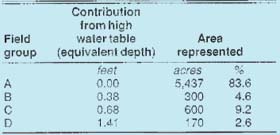

TABLE 2. Optimal irrigation depths, drainwater volumes, and returns to land and management, under a set of drainage policy scenarios
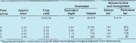
TABLE 3. Optimal irrigation depths, drainwater volumes, and returns to land and management, when a drainwater treatment charge is imposed
Drainwater volume reductions
The best way to reduce district drainwater by 30% involves reducing water applications by 0.84 feet (26%) on farms in all field groups (table 2, policy 2). Such a reduction lowers the drainwater volume by an equivalent depth of 0.21 feet in all field groups, for a 36% reduction on farms without lateral flow contributions and 22,17, and 11% reductions on farms with low, medium, and high contributions from the high water table. Returns to land and management decline by $32 per acre (12%) for all field groups.
A policy requiring that all farms achieve this 30% reduction in drainwater will have a greater economic impact on fields with drainage systems that intercept lateral subsurface flows. Such a policy requires that group A farmers reduce water applications by 0.68 feet (21%), while farmers in groups B and C must reduce applications by 1.24 (39%) and 1.85 feet (58%) (table 2, policy 3). Net returns decline by $23 (9%), $72 (28%), and $159 (62%) per acre in field groups A, B, and C.A 30% drainwater reduction requirement makes production impossible on group D fields, since their contribution from lateral flows exceeds 70% of the initial drainwater volume.
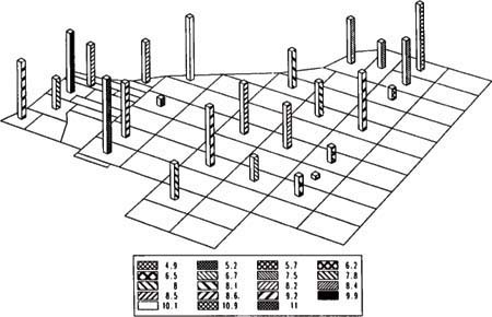
Fig. 1. Average electrical conductivity (EC) in subsurface drainwater samples, Broadview Water District, 1988. The legend indicates average EC (mmhos/cm) of 27 biweekly water samples.
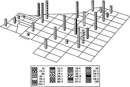
Fig. 1. Volume of drainwater (acre-feet) collected by subsurface drainage systems, Broadview Water District, 1986-1988.
Farmers in group A earn higher returns to land and management under the uniform farm-level plan than under the optimal reduction scheme, since the optimal plan requires a greater reduction in water applications to their fields. Returns to farmers in groups B, C, and D are lower under the uniform restriction than under the optimal plan. These fields require significant reductions in water applications in order to reduce their drainwater by 30%, given their contributions from lateral flows.
Drainwater treatment charges
Charging for drainwater treatment is an alternative that does not involve mandatory reductions in drainwater volume. A treatment charge can raise revenues to pay for drainwater treatment and can motivate farmers to reduce drainwater volumes. Actual treatment costs can be imposed at the farm level as a per-unit charge on collected drainwater, or recovered at the district level through an increase in the price of irrigation water.
A drainwater treatment charge of $100 per acre-foot reduces the returns to land and management by $66 per acre (26%) for all field groups when treatment costs are recovered through an increase in the price of water (table 3). The price of water rises to $42 per acre-foot and the volume of applied water falls by an equivalent depth of 0.28 feet (9%) in all field groups. The alternative, imposing a $100 charge on farm-level drainwater volumes, has important distributional consequences. Net returns for group A fields are $203 per acre when the farmlevel drainwater charge is implemented, but in groups B, C, and D, returns fall to $165, $135, and $62 per acre. A drainwater treatment charge in excess of $130 per acre-foot results in a net loss for group D farms.
Farmers in group A would clearly prefer to pay a drainwater fee at the farm level rather than face an increased water price. Farmers in the other field groups would prefer that the costs of treating the drainwater, including the intercepted lateral flows, be spread evenly across the district through an increase in the irrigation water price.
Conclusions
Farm-level returns to land and management may vary significantly as a result of different approaches to drainwater reduction where a regional high water table contributes to the volume of drainwater collected by individual drainage systems. Policies that require all farms to reduce drainwater volumes by the same proportion may sharply reduce the net returns of growers whose fields receive substantial water from the high water table. Alternative policies would account for the presence or absence of lateral flows, or would implement water pricing schemes that spread the costs of drainwater reduction evenly throughout a district or region.
The cost of administering an optimal drainage reduction plan is an important consideration when selecting a district-level program for drainwater reduction. Measuring drainwater volumes and constituent concentrations in individual drainage systems is often difficult because of the original design of the system, and even when accurate data are available for the complete drainage system, identifying the drainwater volumes that arise from irrigating an individual farm field can be complicated by overlapping ownership of fields drained by a single system. Lateral flows further complicate the situation. In such circumstances, a district-level water pricing policy may be the most effective, economical means of reducing drainwater.
Economics of agricultural drainage policies