Ecosystem services, sometimes called “nature's services,” are broadly defined as the ecosystem functions that benefit people (Daily 1997; Turner and Daily 2008). They are commonly grouped into four categories: supporting, provisioning, regulating and cultural services. Supporting services, such as nutrient recycling and soil formation, allow other ecosystem services to function. Provisioning services include food, raw materials, water and energy. Regulating services, such as carbon sequestration and water purification, regulate ecosystem processes. And cultural services, such as recreational opportunities, contribute to our quality of life. While the economic value of ecosystem services is often debated (Naidoo et al. 2008; Rockström et al. 2009), there is little doubt that the services are essential to human life (Daily 1997).

Often, however, ecosystem services are not taken into account when land use and policy decisions are made (Gómez-Baggethun et al. 2010) — either because the services are difficult to quantify or because they are not thought of as benefits until they are lost (Daily et al. 2009). Loss of ecosystem services can lead to suboptimal landscapes for humans, plants and animals (Nelson et al. 2009). A key challenge for scientists and policymakers is to quantify the values of ecosystem services so that those values, which may be found in both wild and agricultural lands, can be fully accounted for in land-use decisions.

In California, the conversion of land to more intensive uses such as housing threatens the supply and delivery of ecosystem services (Cameron et al. 2014). Since 1984, over 1.4 million acres has been converted from agricultural to other uses, 78% of that to urban development (California Department of Conservation 2011). Various land-use policies exist to manage these conversions, including regulatory zoning and general plans adopted by local governments (Bowers and Daniels 1997). Their effectiveness varies, with policies showing promise in some locations but not others (Butsic et al. 2011; Pogodzinski and Sass 1994).

An alternative to regulatory approaches to land use policy is the purchase, either in fee title or through conservation easements, of private land for conservation (Fishburn et al. 2009; Sundberg 2006). Such transactions may involve local government agencies, private entities such as land trusts or a combination. This approach is common in California, with over 1 million acres conserved by land trusts as of 2010 (Land Trust Alliance 2011). Land conservation may help maintain ecosystem services by preventing conversion of natural and low intensity agricultural land to more intensive uses such as urban, residential or industrial development or large-scale agriculture (Rissman and Merenlender 2008).

The purchase of conservation easements on agricultural land is one approach to preventing residential development on working landscapes. The authors present a low-cost tool for assessing ecosystem service values across large areas, a step toward quantifying the benefits of land conservation.

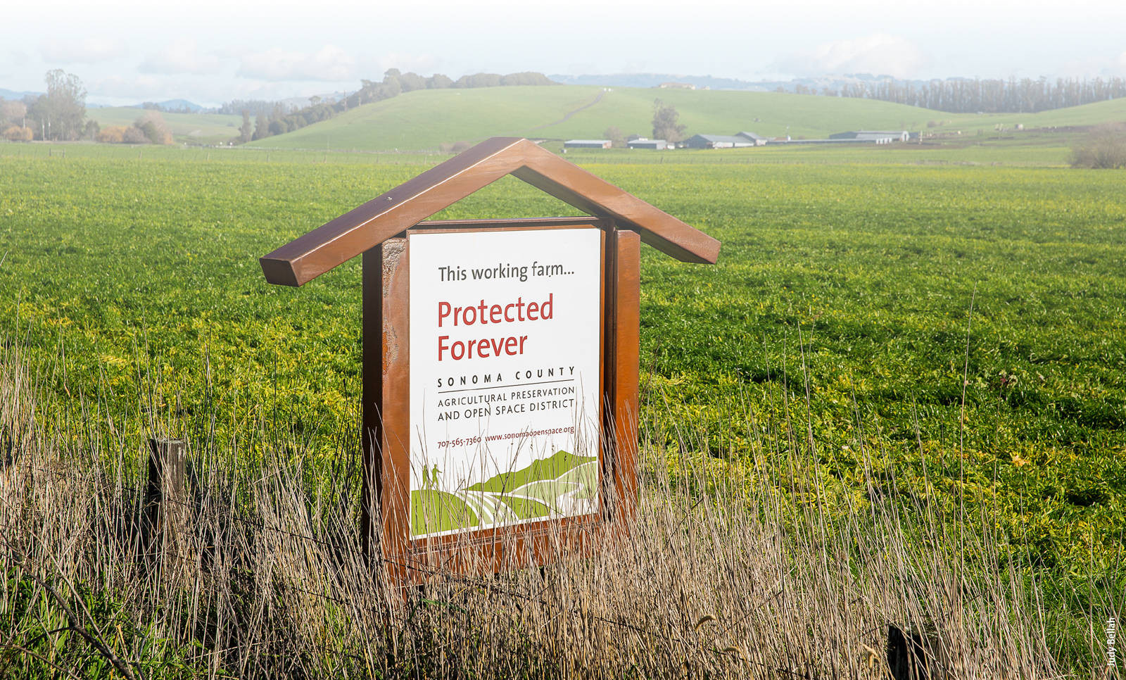
In 1990, Sonoma County residents created the Sonoma County Agricultural Preservation and Open Space District (District) to permanently protect the greenbelts, scenic viewsheds, farms and ranches, and natural areas of the county. Living on the northern edge of the rapidly urbanizing Bay Area, and facing the loss of the natural and agricultural landscapes that define the county's rural character, the voters of Sonoma County recognized the need for proactive local funding for agricultural and open space protection. Voters approved a ballot measure that created the District and instituted a quarter-cent sales tax to fund District operations. The District is now one of the oldest and largest land conservation programs in California; over 100,000 acres has been protected through purchases of land and conservation easements over the last 25 years. Many of the purchased properties are likely to have high ecosystem service values (Ferranto et al. 2011; Plieninger et al. 2012), although these values have not been quantified.

Quantifying ecosystem services can be difficult (Eigenbrod et al. 2010). Models built to assess the biophysical parameters that constitute ecosystem services — such as carbon storage and sediment retention — often require large amounts of spatially explicit data that is not readily available. This issue has limited the application of the ecosystem services concept as a tool to quantify the benefits of land conservation programs, and to help the programs plan for the future (Daily et al. 2009).

Recent advances in modeling techniques, however, in particular the InVEST modular toolset developed by the Natural Capital Project (Sharp et al. 2015), promise to simplify the process of quantifying ecosystem services. The InVEST toolset is designed to run using the many free, large-scale datasets that are available for most California land types, and it can be run on standard personal computers. InVEST can assess the value of 18 different ecosystem services, including carbon sequestration, water yield, nutrient retention, and recreation and tourism. This tool may open the door for widespread quantification of ecosystem services across California.

To quantify the ecosystem services provided by conserved lands in Sonoma County, we used InVEST to estimate carbon storage, sediment retention, nutrient retention (nitrogen and phosphorus) and water yield. We chose these four ecosystem services because of their importance and because they can be degraded by land-use conversions. Carbon sequestration is being monetized in the California carbon markets, and methods to evaluate carbon storage are needed statewide. Land conversions to more developed uses generally reduce carbon on the landscape. Sediment and nutrient retention impact water quality, which is important for human needs and also ecosystem needs; conversions of vegetation often result in poorer water quality. In the current era of drought, water yield from California landscapes is a topic of public concern, as every drop of water becomes more valuable. Land-use conversions can impact the amount of groundwater recharge or loss through runoff.

We quantified the ecosystem services for all of Sonoma County and then summarized the results across three types of land: (1) land purchased by the District, (2) land adjacent to District lands and (3) land that has been converted to developed uses in the last 15 years. While we did not do an economic valuation of each ecosystem service, the values we present here could serve as the foundation for such an analysis.

This process allowed us to test three hypotheses:

1. Do lands conserved by the District have higher ecosystem service values (carbon storage, sediment retention, nitrogen and phosphorus retention, and water yield) than lands adjacent to them or to developed land?

2. How are the ecosystem services correlated across land-use categories? Do high values for one service tend to be associated with low values for another?

3. What are the strengths and weaknesses of using the InVEST toolset at the county scale?

Study area

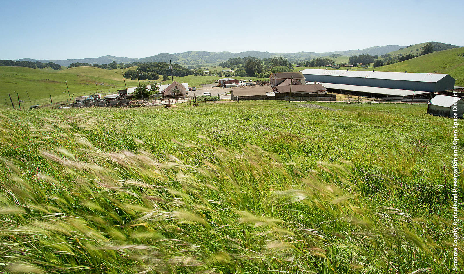
Sonoma County, located on the northwestern edge of the Bay Area, is comprised of roughly 1 million acres of farmland, rangeland, forest, cities and suburbs. It produces some of California's finest wines and cheeses, and its farms and ranches account for roughly 50% of the county's acreage. Forest covers approximately 41% of the county and has a modest impact on the economy (USDA 2016). Urban and suburban development and water constitutes the remaining 9% of the land area. Population has doubled over the last 30 years to nearly half a million people; during that time, over 10% of the best agricultural land (land classified as “Prime Farmland” by California's Farmland Mapping and Monitoring Program) has been converted to more intensive uses, and this trend is likely to continue in the near future.

The study assessed four ecosystem services provided by Sonoma County landscapes: carbon storage, sediment retention, nutrient retention and water yield.

Land typology

We classified the landscape of Sonoma County into three land typologies:

• District lands

• Land adjacent to District land

• Converted lands, lands converted from rangelands or woodlands to development (urban or residential) since 2001.

We classified as District lands all properties that had been acquired by the District since its founding, including parcels that were then managed by agencies other than the District. Lands adjacent to District lands were identified as those that shared a border with District properties, using the “Select” tool in ArcMap (fig. 1). These properties were identified using the Sonoma County parcel data layer rovided by the county.

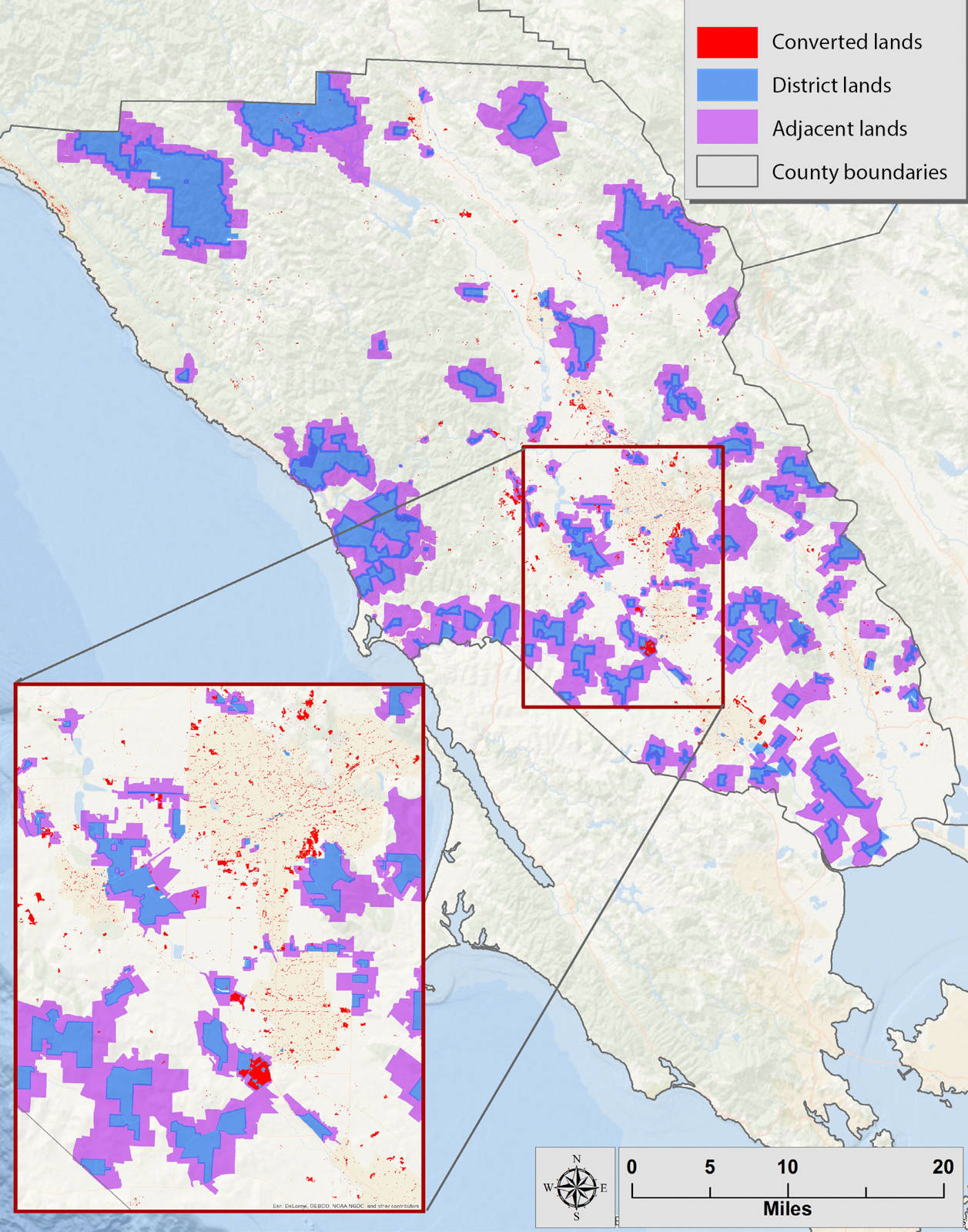
Fig. 1. The study compared the average ecosystem service values of: parcels converted to developed uses in the past 15 years (“Converted land”); parcels conserved by the Sonoma County Agricultural Preservation and Open Space District (“District land”); parcels bordering District lands (“Adjacent lands”); and county lands as a whole.

We believe adjacent lands provide useful points of comparison with district lands. Since they are necessarily in the same geographic area, they would be expected to have similar biophysical features. Likewise, we found mean elevation and slope to be similar between the two types of parcels. District lands had a slope of 16.08 degrees (SD 9.96 degrees) and an elevation of 256.73 meters (SD 168.82 meters); adjacent lands had a slope of 13.85 degrees (SD 9.77 degrees) and an elevation of 222.63 meters (SD 184.61 meters). That said, we do not suppose that adjacent lands are a perfect control. Often, protected lands differ from non-protected lands (Joppa et al. 2008), and we did not attempt to control for these differences by statistical means.

To identify converted lands, we identified change pixels using the 2001–2011 National Land Cover Dataset (NLCD) change product. We identified all nonurban pixels that had converted to developed uses between the years 2001 and 2011. We then identified these pixels on the 2010 LANDFIRE database, the primary vegetation database used in our study.

All data was converted to 30-meter pixels. Using the methods described above, we calculated the total acreage of Sonoma County as 1,060,766 acres; total District holdings as 105,925 acres; adjacent lands to existing District land as 123,600 acres; and converted lands as 7,056 acres.

Evaluating ecosystem services using InVEST

InVEST is a modular, open-source, free toolset in which tabular and spatial data are combined with stand-alone biophysical models to quantify, visualize and compare the delivery of key ecosystem services. While each module is different, most InVEST modules require a base land cover layer, a digital elevation model (DEM) and tabular data that set model parameters for the biophysical models. Outputs describe ecosystem services in terms of their biophysical values and their spatial location (for example, kilograms of carbon stored in a given 30-meter pixel). Full technical descriptions of each module can be found in the module user's guide (table 1). Our description of the models closely follows these guides.

TABLE 1. Data requirements and source information used as inputs in the InVEST modules

InVEST module 1: Carbon storage

The InVEST module uses land cover maps and data on stocks in four carbon pools (aboveground biomass, belowground biomass, soil, and dead organic matter) to estimate the amount of carbon currently stored in a landscape. The estimation of total carbon storage is the sum of all carbon pools for each land cover type. The InVEST result is an estimate of carbon stocks for each pixel on the landscape.

For our model, we use estimates developed by the Nature Conservancy and the District of aboveground carbon associated with LANDFIRE land cover types in Sonoma County (USDA 2013). We used this local dataset as we considered it more accurate than more broad scale carbon estimates, such as estimates published by the Intergovernmental Panel on Climate Change (IPCC). For the belowground carbon pools, the LANDFIRE dataset for Sonoma County includes over 100 land cover types, but documented carbon estimates exist for only seven of these (Pachauri and Meyer 2014). We approximated belowground carbon for the other land cover types by assigning values to these from similar land cover types. Admittedly, this is a source of uncertainty in our results. Another source of uncertainty: we applied an average value for each vegetation type for belowground carbon; therefore, our maps of carbon storage may be inaccurate if there is variation within a land cover type, for instance due to vegetation age. Complete technical details of the model are available from the InVEST user's guide, bit.ly/InvestCS .

InVEST module 2: Sediment delivery ratio

The InVEST sediment delivery model maps overland sediment generation and delivery. Sediment dynamics at the catchment scale are mainly determined by climate (in particular, rain intensity), soil properties, topography, vegetation and anthropogenic factors such as agricultural activities. Sediment sources include overland erosion (soil particles detached and transported by rain and overland flow), gullies (channels that concentrate flow), bank erosion and mass erosion (or landslides).

The sediment delivery module works at the scale of the 30-meter DEM. For each cell, the model first computes the amount of eroded sediment. Eroded sediment was calculated as the annual soil loss, using the Universal Soil Loss Equation (USLE). Data inputs to this equation include rainfall erosivity, soil erodability, slope length gradient factor, crop length factor (specific coefficients accounting for how various crops impact sediment delivery) and support practice factor (impact of alternative conservation practices). Next, the sediment delivery ratio (SDR), which is the proportion of soil loss reaching the catchment outlet, was calculated. The outputs from the sediment model included the sediment load delivered to the stream at an annual time scale, as well as the amount of sediment eroded in the catchment and retained by vegetation and topographic features.

The main limitation of this model was the reliance on the USLE. While this equation is widely used to calculate erodibility, it does not capture all types of erosion and therefore some delivered sediment may not be quantified. Full technical details of this model can be found in the InVEST users' guide, bit.ly/InvestSDR .

InVEST module 3: Nutrient retention

The InVEST Water Purification Nutrient Retention model calculates the amount of nutrient retained on every pixel and sums nutrient export and retention per watershed. The pixel-scale calculations allowed us to represent the heterogeneity of key driving factors in nutrient retention, such as soil type, precipitation and vegetation type.

The model works in three parts. First, annual runoff from each pixel is calculated using the InVEST water yield model. The second phase determines the quantity of nutrient retained by each pixel on the landscape. The model estimates how much pollutant is exported from each pixel based on export coefficients from the user inputs. Export coefficients are annual averages of pollutant fluxes derived from various field studies that measure export from pixels within the United States.

The model was developed for watersheds and landscapes dominated by saturation excess runoff hydrology. The model does not address any chemical or biological interactions that may occur from the point of loading to the point of interest besides filtration by terrestrial vegetation. In reality, pollutants may degrade over time and distance through interactions with the air, water, other pollutants, bacteria or other actors. Full technical details of the model can be found in the InVEST user's guide, bit.ly/InvestNR .

InVEST module 4: Water yield

InVEST maps and models the annual average water yield from a landscape, defined as the amount of water running off the landscape. The model runs on a gridded map, estimating the quantity of water for each subwatershed in the area of interest. First, it determines the amount of water running off each pixel as the precipitation less the fraction of the water that undergoes evapotranspiration. The model does not differentiate between surface, subsurface and baseflow, but assumes that all water yields from a pixel reach the point of interest via one of these pathways. This model then sums and averages water yield to the subwatershed level. The pixel-scale calculations allow us to represent the heterogeneity of key driving factors in water yield, such as soil type, precipitation and vegetation type. However, the theory we are using as the foundation of this set of models was developed at the subwatershed to watershed scale. We are only confident in the interpretation of these models at the subwatershed scale, so all outputs were summed and/or averaged to the subwatershed scale. Technical details of the water yield model can be found online at bit.ly/InvestWY .

The type of vegetation cover influences the value of all four of the ecosystem services assessed in the study.

Combining and comparing services

To understand the spatial distribution of the ecosystem services, we mapped the values of each (figs. 2A–E). We also developed a map of “hotspots” — areas that have high values for most or all services assessed (fig. 3) — using the following method. First, we rescaled the pixel level ecosystem services by dividing each pixel value by the maximum value for that service. This created a scaled raster for each service with a maximum value of 1. We then added the raster values from all services to create a map in which the maximum value of each pixel was 5. That is, if a pixel had the maximum value for all five services, it would have a value of 5.

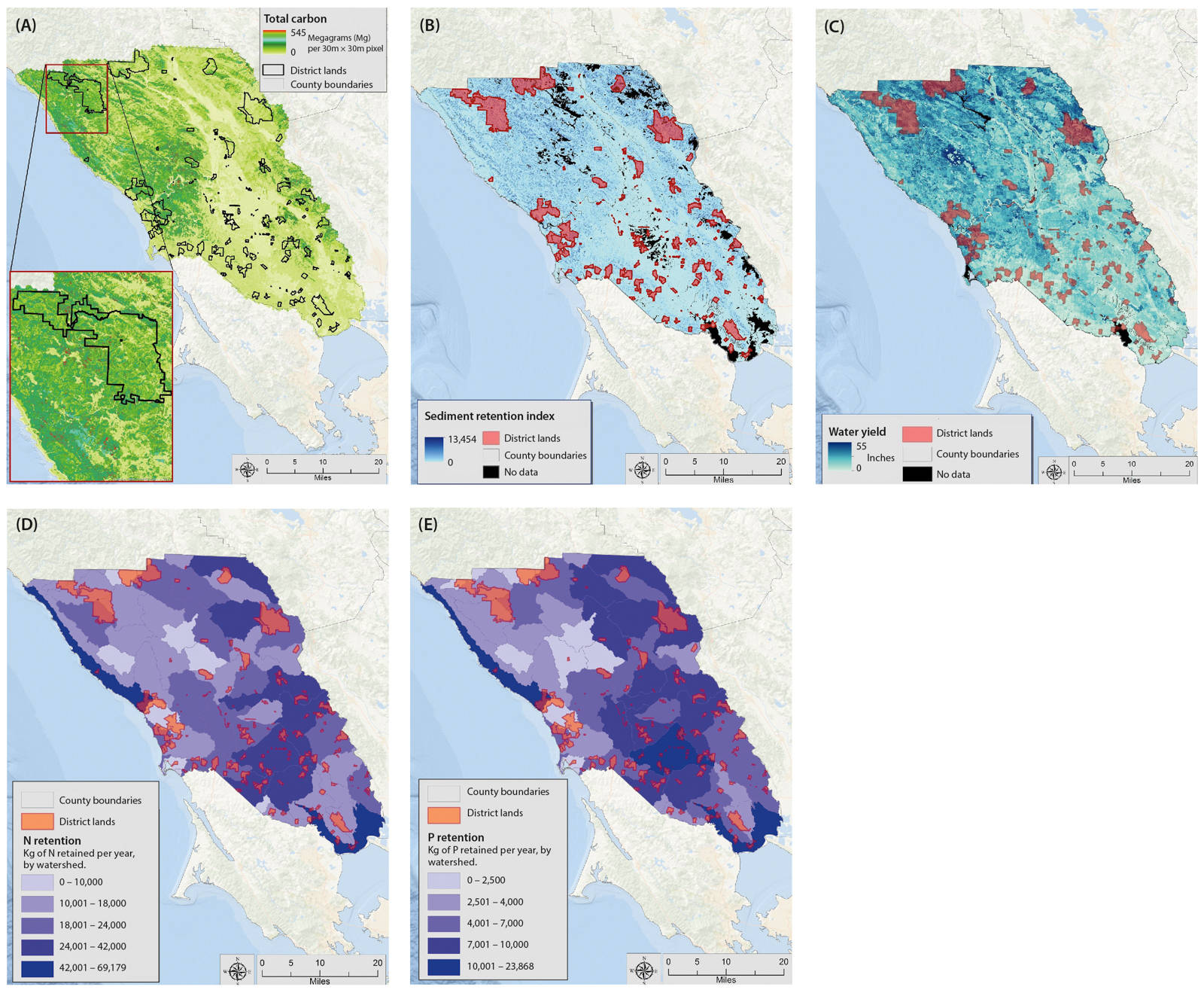
Fig. 2. Map of (A) total carbon storage, (B) sediment retention index, (C) water yield, (D) nitrogen retention and (E) phosphorus retention.

Fig. 3. Combined index of the ecosystem service values shown in Fig. 2 A–E.

To compare the potential trade-offs among ecosystem service values within different land types — that is, the positive or negative correlations — we created spider graphs (fig. 4). These graphs show the scaled value for the mean of each service for each land typology. For example, if District lands had the highest mean carbon per acre, on the spider graph District land would receive a 1.0. If adjacent lands had a mean carbon value of 60% of the District lands, they would be represented by a 0.6 on the spider graph, and so forth.

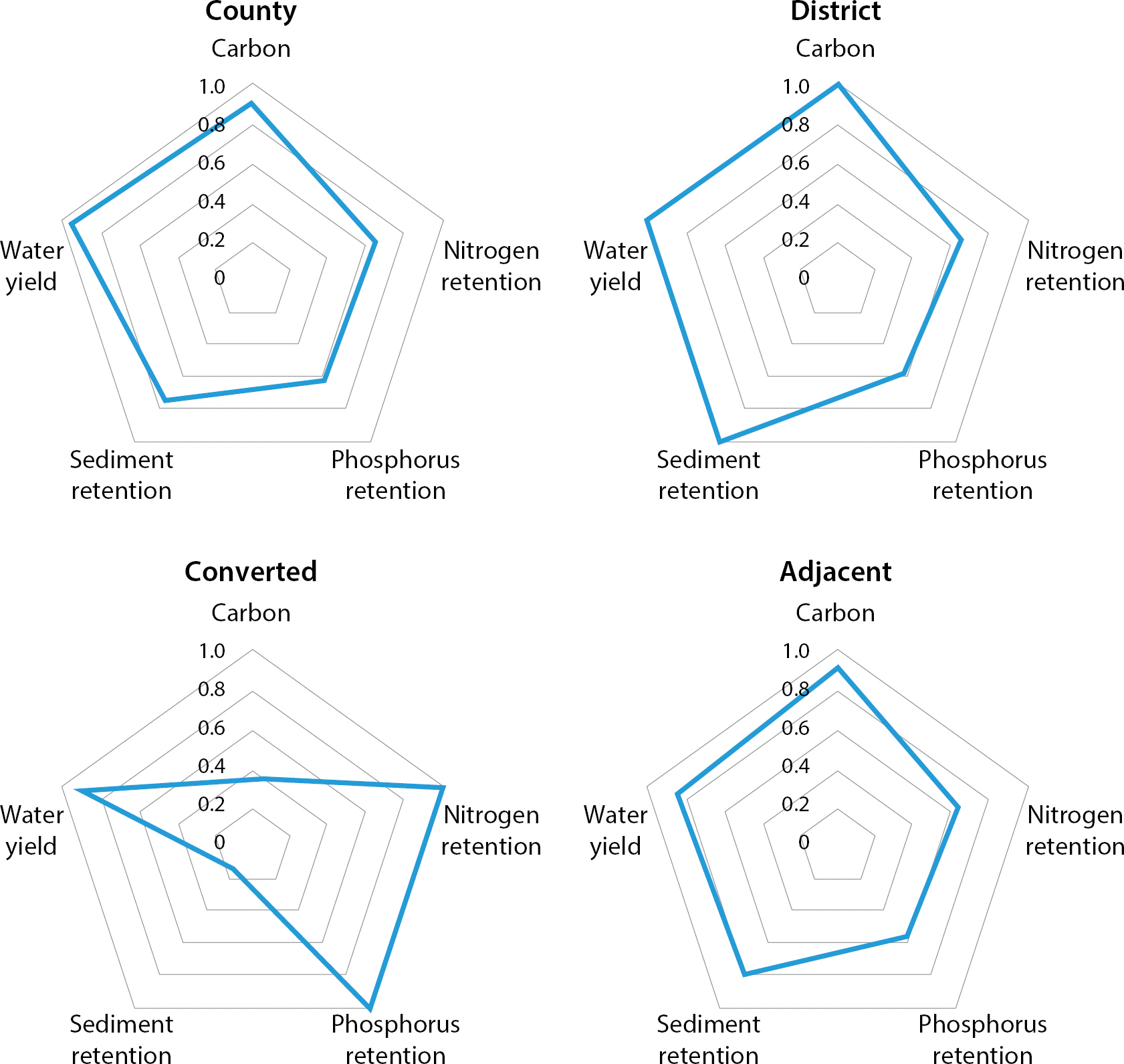
Fig. 4. Spider diagrams show the trade-offs among ecosystem service values across the four land categories studied.

Model results

Carbon storage

Our models estimate carbon storage in Sonoma County at 205,496,048 Mg (fig. 2A). About 10.5% of carbon storage occurs on District lands, and District lands have the highest mean carbon storage levels, with an average of 49 Mg per pixel compared to 45 Mg for the county and 16.54 Mg for converted lands. The per-pixel level of carbon storage is primarily driven by vegetation type, and hence follows a gradient: developed land uses have lowest carbon storage levels, and forested areas with high biomass have the highest levels (table 1, fig. 2A).

Sediment retention

The sediment retention index is a comparison of the potential for soil loss from a given pixel without vegetation versus with current vegetation (fig. 2B). High values indicate that more soil loss is prevented due to vegetation. District lands rank high; the vegetation on these lands does a good job of retaining sediment, especially considering the high potential that these areas have for sediment export given their high average slope. County lands and adjacent lands rank lower, but both are far ahead of converted lands (table 2).

TABLE 2. Summary of model results

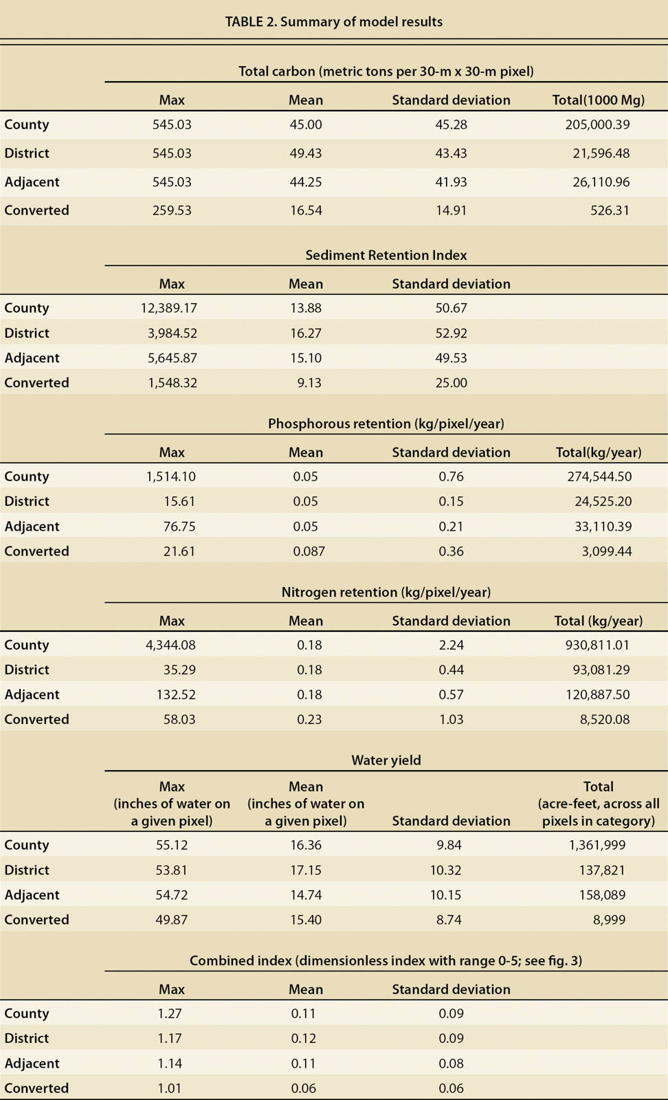
The sediment retention model produced six results, one of which we report here. We computed the potential soil loss per pixel, calculated with the current land cover, indicating the potential for soil loss from each land typology. District lands are vulnerable to soil loss; partially due to steep gradient lands, whereas converted lands have low potential for erosion; primarily because many of the conversions take place in areas that are relatively flat (table 2).

Nutrient retention

Converted lands retained the most phosphorous, on a per-unit basis (fig. 2D). As with sediment retention, converted lands have low potential to export nitrogen and phosphorous, due to their generally flat topography (table 2). At the watershed scale, we see maximum retention in the low-lying areas around San Pablo Bay, in the southern portion of the county. Nitrogen retention follows a very similar pattern with highest retention rates near San Pablo Bay.

Water yield

District properties had the highest per-cell water yield, followed by the county and converted lands (fig. 2C). Interestingly, District lands had an almost 15% higher water yield than the parcels adjacent to them. Per-pixel water yield follows both a rainfall and vegetation gradient across the county (table 2). Maximum water yield occurs in steeper areas in the northern half of the county.

Combined services index

The map of the combined ecosystem services index (fig. 3) shows that District lands tend to have relatively high values (table 2). It also shows that most parcels were not able to supply high levels of all ecosystem services. For the services analyzed, lands in the forested northwest of the county tend to have the highest combined ecosystem service values and the district has focused significant effort on purchasing these lands. The spider diagrams reveal that County and District lands rank relatively high in all ecosystem services. Converted lands rank lowest in carbon sequestration and sediment retention properties, as would be expected. The spider graphs illustrate how no one type of parcel provides the highest level each ecosystem services. This indicates that there are trade-offs between conserving different services.

Utility of the InVEST toolkit

Land is often conserved with the idea that conservation will protect ecosystem services, although these services are rarely quantified. Our analysis found that District lands provide higher levels of the ecosystem services studied, based on a composite index, than lands adjacent to District lands, converted lands and county lands overall. However, because we did not do a counterfactual analysis, we cannot say whether the District's land and easement purchases are responsible for these higher values. If the District purchased lands that would not have developed even in the absence of conservation, the impact of District purchases may be modest; though it is also possible that the lands would have been managed differently if they had not been purchased.

The map of ecosystem service hotspots highlights areas in the county with high composite ecosystem service values. District purchases in these areas may result in high ecosystem service conservation. While the bulk of hotspots are in forested areas in the northern part of the county, there are high-value pockets throughout the county, indicating that the District may be able to choose from a suite of high ecosystem service parcels.

Our results are dependent on the suite of ecosystem services we selected. In our case, carbon storage and sediment retention are highest in forested areas, and therefore, our analysis values this vegetation type most highly. If other ecosystem services were selected, for example food production or pollination services, the results might have been different. For results such as these to be useful for policy purposes, one must be sure that the ecosystem services evaluated fit the priorities of the communities in question.

From a methodological perspective, InVEST was a useful tool, capable of quantifying ecosystem services across broad scales, and making use of public datasets that are freely available for most or all of the state.

There was no way to directly validate our results. Other ecosystem service quantification efforts in Sonoma County that we are aware of, such as the aboveground carbon estimates produced by the District and The Nature Conservancy, were used as inputs in our analysis, and therefore could not be used for validation purposes. Linking external validation to InVEST estimates would be a useful extension of our research. However, this would require alternative models that also predict these services. With the possible exception of some alternative carbon sequestration models (Gonzalez et al. 2015), such models do not exist.

However, given that we are most interested in using InVEST for management actions which will rely on comparing ecosystem services within the same study area, we suspect that the relative values produced by InVEST will be useful to managers. Although the actual ecosystem service values may suffer from some inaccuracy, we suspect that the relative values of parcels within our study area may be similar. In this way, even if ecosystem services estimates are not completely accurate, they still may be useful for comparing competing sites in our study area.

An obvious extension of this work would be calculating the economic value of the ecosystem services. This could be accomplished by a host of methods, including benefits transfer, hedonic models or contingent valuation. In addition, quantifying the impacts of District land and easement purchases on ecosystem services would be interesting. We know of some landowners who have used District payments to purchase more land for agricultural use, thus providing a potential double benefit of district purchases. Quantifying how common this type of action is would give a more complete view of the total benefits generated by District land conservation expenditures.

Protecting ecosystem services while communities grow will remain a challenge across California. Purchases of private land for public use will likely continue to be a popular nonregulatory method for constraining land use. Choosing the best sites to purchase will likely be a continued area of debate. Consistent quantification of ecosystem services can help communities make better land-use decisions. Given the difficulty of assessing ecosystem values, InVEST may prove to be a useful toolset for this purpose.