California Agriculture
University of California
California Agriculture

All Issues

Statistical analysis of monitoring data aids in prediction of stream temperature

Share using any of the popular social networks Share by sending an email Print article

Authors

Kenneth W. Tate , UC Davis;
David Lile, Lassen County;
Donald L. Lancaster, UCCE Modoc County;
Marin L. Porath, Lakeview County
Julie A. Morrison, Idaho Cattle Association
Yukako Sado, UC Davis

Publication Information

California Agriculture 59(3):161-167. https://doi.org/10.3733/ca.v059n03p161

Published July 01, 2005

PDF  |  Citation  |  Permissions

Author Affiliations show

Abstract

Declines in cold-water habitat and fisheries have generated stream-temperature monitoring efforts across Northern California and the western United States. We demonstrate a statistical analysis approach to facilitate the interpretation and application of these data sets to achieve monitoring objectives. Specifically, we used data collected from the Willow and Lassen creek watersheds in Modoc County to demonstrate a method for identifying and quantifying potential relationships between stream temperature and factors such as stream flow, canopy cover and air temperature. Our monitoring data clearly indicated that a combination of management practices to increase both in-stream flow and canopy cover can be expected to reduce stream temperature on the watersheds studied.

Full text

IN our previous paper on graphical analysis ( see page 153 ), we utilized a 3-year stream-temperature data set — collected from the Lassen and Willow creek watersheds in northeastern Modoc County (in the northeastern-most corner of California) — to demonstrate graphical analysis approaches to reduce, display and interpret a typical large, raw stream-temperature data set. In this paper, we report the results of statistical analysis conducted on this same data set, to identify and quantify relationships between stream temperature, air temperature, stream flow, stream order and riparian canopy cover.

Stream-monitoring efforts typically produce data sets composed of temperature readings (such as hourly, daily) from a set of discrete locations across a stream system. These cross-sectional, longitudinal surveys — in which a cross-section of available locations is monitored over time (longitudinal) — are common across Northern California and the West. To optimize the analysis and interpretation of such stream-temperature data sets, we believe it is critical to collect data on associated factors such as air temperature, stream flow and stream canopy for each location. To identify and quantify relationships between stream temperature (the dependent variable) and associated factors (the primary independent variables), we propose a regression-based analysis approach.

Regression analysis can be applied to data to determine, for predictive purposes, the degree of correlation of a dependent variable with one or more independent variables. The objective is to see if there is a strong or weak relationship.

In this case, we developed a linear equation (model) that displayed the estimated effect of several independent variables on the dependent variable, stream temperature. The simple form of the equation is:y = a + (b1X1) + (b2X2)+…+(biXi) where y is the dependent variable, a is the intercept of the equation, b1 is a coefficient that estimates the relationship between the independent variable X1 and the dependent variable y, given that the other factors (X2,3… i) are also present in the model. The model coefficients (bi) represent the best-estimate identification and quantification of the relationships between stream temperature (y) and the factors of interest (Xi).

A 3-year monitoring data set was collected from watersheds in Modoc County in order to demonstrate approaches for displaying and analyzing stream-temperature and related data in meaningful ways. Left, a densiometer is used to estimate the percentage of vegetative canopy cover over a stream. Above, willows (foreground) and aspen (background) budding in early spring will provide shade cover to reduce temperatures during the summer.

A 3-year monitoring data set was collected from watersheds in Modoc County in order to demonstrate approaches for displaying and analyzing stream-temperature and related data in meaningful ways. Left, a densiometer is used to estimate the percentage of vegetative canopy cover over a stream. Above, willows (foreground) and aspen (background) budding in early spring will provide shade cover to reduce temperatures during the summer.

This approach is not a definitive test of cause and effect, as would be expected in a controlled experiment. However, experimental tests of how associated factors affect stream temperature, particularly at the watershed scale, are generally impractical due to the lack both of “replicate” streams and of experimental control over the independent variables. Caution must be taken in the development and interpretation of regression models examining relationships between stream temperature (y) and associated factors (Xi). As with any analysis, the results are only as good as the data used. The appropriateness of the monitoring locations selected (e.g., are the locations representative of the stream system, watershed or region?) and data collection methods must be considered.

Stream-temperature monitoring locations on Lassen, Willow and Cold creeks in northeastern Modoc County, Calif.

Fig. 1. Stream-temperature monitoring locations on Lassen, Willow and Cold creeks in northeastern Modoc County, Calif.

The authors calculated the significance and 95% confidence intervals of the coefficients for each independent variable associated with daily maximum stream temperature, including stream flow and canopy cover on Lassen Creek, above.

The authors calculated the significance and 95% confidence intervals of the coefficients for each independent variable associated with daily maximum stream temperature, including stream flow and canopy cover on Lassen Creek, above.

It is important to confine conclusions drawn from regression analysis only to the factors that were examined for inclusion in the final model (e.g., conclusions about the importance of stream flow relative to air temperature can be drawn only if both factors were examined simultaneously). A good rule is to examine if the relationships make sense in light of existing knowledge and basic principles. If the relationship is not readily explainable, then additional research or monitoring is warranted to refute or confirm it.

Regardless of the analysis approach used, the potential effect introduced by repeatedly measuring stream temperature at each monitoring location must be considered. A basic assumption of many statistical analysis techniques is that each observation in the data set is independent of all other observations in the data set. However, it is unlikely that the daily maximum stream temperature at monitoring location W1 (fig. 1) on June 15 is independent of the daily maximum stream temperature at this location on July 1. This problem is typical of most longitudinal data sets (repeated measurement at a fixed site through time). The codependence introduced by repeated measurements of a single location through time can be addressed using a linear mixed-effects regression analysis (Pinheiro and Bates 2000), which we employ in this paper, or other approaches such as a repeated-measures analysis of variance.

Statistical analysis of data

The dependent variable that we analyzed was daily maximum stream temperature (oF) collected at numerous fixed dates across the summer, at fixed sites across the Lassen and Willow creek watersheds (fig. 1). We selected daily maximum as an example because it is a simple and biologically important measure of cold-water habitat; however, the same analysis could be conducted on other metrics of interest, such as 7-day running average of daily maximum stream temperature or change in maximum stream temperature per stream mile ( see page 153 ). The maximum stream temperature for each 24-hour time period from June 15 through Sept. 15, in 1999, 2000 and 2001 was extracted from the half-hour time series of data at each of 22 monitoring locations (see fig. 1). To further reduce the data set, we used the daily maximum stream temperature at each site for June 15, July 1, July 15, Aug. 1, Aug. 15, Sept. 1 and Sept. 15 from each year as the dependent variable (n = 462 observations).

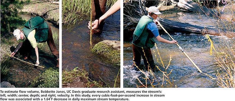
To estimate flow volume, Bobbette Jones, UC Davis graduate research assistant, measures the stream's: left, width; center, depth; and right, velocity. In this study, every cubic-foot-per-second increase in stream flow was associated with a 1.64 F decrease in daily maximum stream temperature.

To estimate flow volume, Bobbette Jones, UC Davis graduate research assistant, measures the stream's: left, width; center, depth; and right, velocity. In this study, every cubic-foot-per-second increase in stream flow was associated with a 1.64 F decrease in daily maximum stream temperature.

Graphical analysis of this data set (in our previous figs. 2 and 3, page 156) clearly illustrated that stream temperature increases to a peak in July and August and decreases in September. For this statistical analysis, we selected bimonthly data from the larger continuous daily maximum stream temperature data set in order to capture the evident seasonal pattern in temperature while limiting data redundancy. Depending upon the monitoring and analysis objectives, alternative approaches could be the use of weekly or monthly calculations (e.g., average or maximum) across the summer or the use of all daily maximum stream temperature records.

The linear mixed-effects analysis (Pinheiro and Bates 2000) conducted on bimonthly daily maximum stream temperature from locations on Lassen, Willow and Cold creeks contained the following fixed-effect independent variables: date (June 15, July 1, and so on), daily maximum air temperature (°F), stream flow (cubic feet per second [cfs]) and stream canopy cover (percentage of sky blocked by vegetation) of the 1,000-foot reach upstream of the site (DFG 1998). Daily maximum air temperature for each date from the nearest air-temperature monitoring location was matched to each stream-temperature observation. Additional terms introduced in the initial model included all possible interactions among independent variables as well as the quadratic form of all continuous variables (air temperature, stream flow and canopy cover). An interaction occurs when the effect of one independent variable on y depends upon another independent variable. Including the quadratic form (Xi2) of each continuous independent variable allows for the potential that the relationship between x and y is not a straight line.

To account for each location's position in the watershed, stream order for each monitoring location was introduced as an independent variable. A headwater channel is a first-order stream, the merger of two first-order channels forms a second-order stream, and the merger of two second-order channels forms a third-order stream. Monitoring location identity and year (1999, 2000 and 2001) were treated as random effects to account for repeated measures and for random variations in annual weather, respectively. A backward stepwise approach was followed until only significant (P ≪ 0.05), factors remained in the model. Insignificant main effects were left in the model if interaction terms containing the main effect were significant. For example, if the interaction term for stream flow and air temperature was significant (P ≪ 0.05), then both stream flow and air temperature were retained in the model regardless of their significance. The evaluation of residual error plots indicated that assumptions of normality, independence and constancy were met.

Model predicts stream temperature

The evaluation and interpretation of statistical models require the display of several important outputs, including: (1) the final statistical model with coefficients, coefficient confidence intervals and significance levels for all variables; (2) the display of the “fit” of the model, or how the model predictions compare with the observed data; and (3) the graphical display of relationships between the independent and dependent variables reported in the final statistical model. The evaluation and interpretation of the statistical model and the relationships that it implies should always be coupled with local knowledge of the system modeled and the application of basic scientific principles. Basically, do the results make sense in terms of accepted principles of hydrology, ecology, and so on? If not, is there a logical explanation that could be tested?

We calculated the significance (P) and 95% confidence intervals of the coefficient estimated for each independent variable associated with daily maximum stream temperature (table 1). The coefficient value indicates the estimated effect (positive or negative) and magnitude of the relationship between each variable and daily maximum stream temperature. For continuous variables (canopy cover, daily maximum air temperature and stream flow), the coefficient indicates the change in daily maximum stream temperature expected with each incremental change in the variable, given that all other factors are held constant. For example, in our case study a 1 cfs increase in stream flow was associated with 1.64°F reduction in stream temperature.

Linear mixed-effects analysis predicting daily maximum stream temperature (‘F) on Willow, Lassen and Cold creeks, June-Sept., 1999–2001*

TABLE 1. Linear mixed-effects analysis predicting daily maximum stream temperature (‘F) on Willow, Lassen and Cold creeks, June-Sept., 1999–2001*

Equation 1

Daily maximum stream temperature (°F)

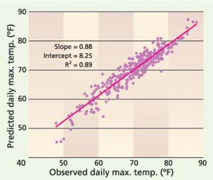
Observed versus predicted daily maximum stream temperatures, as calculated by linear mixed-effects model containing independent variables of stream flow, canopy cover, daily maximum stream temperature and stream order. The model was developed with data collected in 1999, 2000 and 2001 at 22 stream locations on Lassen, Willow and Cold creeks in northeastern Modoc County.

Fig. 2. Observed versus predicted daily maximum stream temperatures, as calculated by linear mixed-effects model containing independent variables of stream flow, canopy cover, daily maximum stream temperature and stream order. The model was developed with data collected in 1999, 2000 and 2001 at 22 stream locations on Lassen, Willow and Cold creeks in northeastern Modoc County.

For categorical variables (stream, date and stream order), the coefficient represents the estimated difference between the referent level and other variable levels, given that all other variables are held constant. The referent level for a categorical variable is the level to which other levels for that variable are compared. The coefficient for the referent level (stream = Willow Creek, date = June 15, stream order = first) was set to zero. The coefficients for other levels represent the estimated difference in daily maximum stream temperature between each level and the referent level. For example, the referent level for “stream” was Willow Creek, and Lassen and Cold creeks were estimated to be 4.43°F and 10.16°F colder than Willow Creek, respectively (table 1).

The coefficients reported in table 1 may be more easily conceptualized as equation 1 (see box). The fit of the statistical model reported in table 1 can be evaluated graphically in figure 2. We used simple linear regression of the form “predicted = a + b x observed” to evaluate the fit of the model. If the model perfectly predicted observed stream temperature, the slope (b) of the regression would equal 1.0 with an R2 of 1.0. Figure 2 indicates that the model in table 1 is not perfect, but with a slope of 0.88 and an R2 of 0.89, it certainly is a reasonable fit.

Interpreting, presenting model

A simple graphical display of this statistical model can facilitate the interpretation and presentation of the results to audiences with limited statistical backgrounds, which can in turn help to achieve monitoring or restoration objectives. Figures 3 and 4 illustrate the use of the statistical model reported in table 1 and equation 1 to “predict” or display the relationships identified between daily maximum stream temperature and significant environmental and management factors. These figures also illustrate the potential to use equation 1 to examine “what if” scenarios, such as the benefit of increasing canopy cover versus stream flow on second-order streams. Such speculation should be limited to the range of the data used to develop the model.

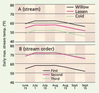
Relationship of daily maximum stream temperature and (A) stream (Willow, Lassen, Cold) and (B) stream order (first, second, third) across the summer season, developed from linear mixed-effects analysis of data from 1999, 2000 and 2001. Other significant factors are set to fixed values: stream order = first (A), stream = Lassen (B); canopy cover = 25%, daily maximum air temperature = 85°F, and stream flow = 2 cfs.

Fig. 3. Relationship of daily maximum stream temperature and (A) stream (Willow, Lassen, Cold) and (B) stream order (first, second, third) across the summer season, developed from linear mixed-effects analysis of data from 1999, 2000 and 2001. Other significant factors are set to fixed values: stream order = first (A), stream = Lassen (B); canopy cover = 25%, daily maximum air temperature = 85°F, and stream flow = 2 cfs.

Relationship of daily maximum stream temperature and (A) stream flow (cfs), (B) stream canopy cover (%) and (C) daily maximum air temperature (°F), across the summer season, developed from mixed-effects analysis of data from 1999, 2000 and 2001. Other significant factors are set to fixed values: stream = Willow; date = Aug. 1; stream order = first (A and C) and second (B); daily maximum air temperature = 85°F (A and B); and stream flow = 2 cfs (C).

Fig. 4. Relationship of daily maximum stream temperature and (A) stream flow (cfs), (B) stream canopy cover (%) and (C) daily maximum air temperature (°F), across the summer season, developed from mixed-effects analysis of data from 1999, 2000 and 2001. Other significant factors are set to fixed values: stream = Willow; date = Aug. 1; stream order = first (A and C) and second (B); daily maximum air temperature = 85°F (A and B); and stream flow = 2 cfs (C).

Stream

Figure 3 A displays the relationship between stream (Lassen, Willow and Cold creeks) and daily maximum stream temperature over the summer season. This relationship was identified and quantified, given that all other significant variables (table 1) were constant and accounted for. In order to generate figure 3A, we set stream order at first, canopy cover at 25%, daily maximum air temperature at 85°F and stream flow at 1 cfs. We then used equation 1 (the statistical model) to estimate daily maximum stream temperature for each stream at each date (fig. 4). Figure 3A is in agreement with raw data presented in our previous article (see figs. 2 and 3, page 156), which illustrated that Willow Creek was on average 4.43°F warmer than Lassen Creek for daily maximum stream temperature. It is also clear that Cold Creek is aptly named, being on average 10.16°F cooler than Willow Creek for daily maximum stream temperature. The seasonal pattern from June through September was also captured with this statistical model.

Stream order

Figure 3B displays the relationship between stream order and daily maximum stream temperature over the course of the summer. It is no surprise that first-order (headwater) stream locations are significantly cooler than second- and third-order locations in the middle to lower reaches of these watersheds. In general, stream temperature will progressively increase from the upper to lower reaches of a stream system, as was the case for all but one reach of Willow Creek (see figs. 2 and 3, page 156). Daily maximum stream temperature was not different between second- and third-order stream locations, given that all other factors were equal. It is clear that the primary sources of cold-water habitat within these streams, as with most, are in headwater locations.

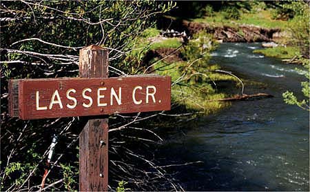
Spring bud break and the onset of leaf set and shade are delayed in the higher elevation reaches of Lassen Creek, while the peak snow melt generates significant stream-flow volumes.

Spring bud break and the onset of leaf set and shade are delayed in the higher elevation reaches of Lassen Creek, while the peak snow melt generates significant stream-flow volumes.

Don Lancaster, UCCE Modoc County natural resources advisor, monitors the stream temperature of lower Willow Creek in the late summer, when its flow volume is lowest.

Don Lancaster, UCCE Modoc County natural resources advisor, monitors the stream temperature of lower Willow Creek in the late summer, when its flow volume is lowest.

Lassen Creek provides critical spawning habitat for several native fish species; temperatures over 77°F can be lethal to salmonids, while sublethal temperatures (67°F to 76°F) can affect growth and spawning.

Lassen Creek provides critical spawning habitat for several native fish species; temperatures over 77°F can be lethal to salmonids, while sublethal temperatures (67°F to 76°F) can affect growth and spawning.

Stream flow

Figure 4 A displays the relationship identified between stream flow (cfs) and daily maximum stream temperature for the Lassen and Willow creek watersheds, which have summer stream flows ranging from 1 to 5 cfs. For every cubic foot per second (cfs) increase in stream flow at a site, there was an estimated 1.64°F decrease in daily maximum stream temperature (table 1). This is an important result, given that one of the suspected sources of elevated stream temperatures is the diversion of stream flow for irrigation.

This result provides local irrigation managers and water-resources professionals with tangible evidence that investments in reducing stream-flow withdrawal demands (e.g., improving the efficiency of irrigation delivery, and matching irrigation amounts and timing to plant water demand and current soil moisture status) will result in reduced daily maximum stream temperatures, as well as reasonable expectations of the likely magnitude of these reductions. The lack of significance of the interaction term for stream flow and stream order (P> 0.05) in this model indicates that the relationship between stream flow and daily maximum stream temperature was constant from the upper to lower reaches of these streams.

This is interesting, given that the sources of increased stream flow in the upper reaches are likely natural phenomena (e.g., the return of subsurface stream flow to the surface, or diffuse springs), while increased stream flow in the lower reaches is likely due partly to warm irrigation-water returns. One might expect increased stream flow in the lower reaches to be associated with increased stream temperatures. However, if a significant portion of irrigation return flow is reaching the stream as cool subsurface flow, then the relationship identified in this analysis is plausible (Stringham et al. 1998).

These statistical results agree with our graphical analysis, reporting relatively low rates of change in stream temperature across the lower reaches of Willow and Lassen creeks (see fig. 4, page 158 ).

Canopy cover and air temperature

There was a significant interaction between stream canopy cover and daily maximum air temperature (table 1), which requires the relationships between stream canopy cover, air temperature and stream temperature to be discussed together for proper context. For every 1% increase in canopy cover in the 1,000-foot reach above a site, there was an estimated 0.15°F reduction in daily maximum stream temperature at that site (fig. 4B). This relationship is logical, given that a reduction in the amount of solar energy reaching a stream's surface should result in a reduction in its temperature.

For every 1°F increase in daily maximum air temperature, there was an expected 0.1°F to 0.8°F increase in daily maximum stream temperature (fig. 4C). This range exists because the relationship is not a straight line as indicated by the significance of the quadratic term ([max. air temp.]2) in the final model (table 1). This quadratic relationship is revealed in the curve of the lines plotted in figure 4C. Basically, the rate of stream-temperature increase associated with rising air temperature is reduced as air temperature increases from 60°F to 90°F (fig. 4C). This is an important relationship in determining the background, or natural, temperature regime for streams in arid, hot regions of the western United States.

The significant interaction between air temperature and canopy cover illustrates the complex relationships between environmental and management variables that determine stream temperature (table 1). As daily maximum air temperature increased, the cooling effect of canopy cover increased (fig. 4C), with the implication that increased canopy cover is more effective at reducing daily maximum stream temperature as air temperature increases. This provides evidence that increasing riparian vegetation and thus stream canopy cover can be expected to reduce daily maximum stream temperature. Most importantly, these results provide local managers with information about the expected reductions that could occur by using vegetation management as a restoration tool, allowing realistic expectations regarding the potential to create cold-water habitat simply by increasing canopy cover alone. For instance, a combination of increased canopy cover and stream flow may generate greater stream-temperature reductions than either practice by itself. It is also important to realize that there are natural limits on the amount of canopy cover and stream flow that each stream reach can generate (e.g., in meadows compared to canyon reaches).

Support for local decision-making

While the relative temperatures of Willow, Lassen and Cold creeks may be of little concern outside of northeastern Modoc County, being able to clearly and defensibly identify warm or cold streams is important for determining possible regulatory actions, allocating limited restoration funds and making other controversial decisions locally across Northern California and the western United States. Stream-temperature monitoring can provide a significant amount of information for making decisions about management changes and restoration projects in order to increase or improve cold-water habitat in streams. On a watershed or regional scale, information about the relationships between stream temperature and factors such as stream canopy cover, stream flow and watershed position are important for identifying and quantifying the expected benefits of practices to reduce stream temperature. For instance, monitoring data presented in this paper clearly indicates that a combination of management practices to increase both in-stream flow and canopy cover can be expected to reduce stream temperature on the watersheds studied.

Practices such as the modification of irrigation and riparian grazing management come with real costs to managers, and decisions to implement these practices should be based on reasonable expectations of the return on that investment in terms of improving cold-water habitat. The monitoring data presented here also places constraints on the expected extent of cold-water habitat given seasonal patterns, air temperature and the position of the stream in the watershed, regardless of increases in canopy cover and stream flow. Collectively, these results provide local information required for watershed groups to reach a balance between restoration desires, management possibilities and inherent environmental constraints.

On this meadow reach of mid-Lassen Creek, shade from willows is naturally low. The data collected indicates that management practices to increase stream flow and canopy cover can bring down stream temperatures in areas where logging, stream diversions and other uses have caused them to increase.

On this meadow reach of mid-Lassen Creek, shade from willows is naturally low. The data collected indicates that management practices to increase stream flow and canopy cover can bring down stream temperatures in areas where logging, stream diversions and other uses have caused them to increase.

For monitoring data to be interpreted and integrated into restoration plans, regulatory processes and land-use management decisions, data must be appropriately collected and analyzed. In our previous paper, we illustrated the value of simple graphical analysis to address certain typical stream-temperature monitoring objectives. In this paper, we illustrated the potential of using relatively simple statistical analysis to achieve additional monitoring objectives and information needs. It is important to examine and plan for data analysis options during the initial development of the monitoring plan prior to data collection, not only after the data has been collected. While most individuals and groups planning and conducting monitoring may not have the statistical expertise to conduct the analysis described here, such support is available within many state and federal agencies and organizations (both regulatory and nonregulatory) to assist with monitoring plan development, implementation and analysis. Many such agencies are active members of local and regional restoration, conservation and watershed groups, including UC Cooperative Extension, the U.S. Department of Agriculture Natural Resources Conservation Service, the California State Water Resources Control Board, the California Regional Water Quality Control Boards and the California Department of Fish and Game.

Return to top

References

[DFG] California Department of Fish and Game. California Salmonid Stream Habitat Restoration Handbook. Appendix M 1998. Sacramento, CA: http://www.dfg.ca.gov/nafwb/manual.html .

Pinheiro JC, Bates DM. Mixed Effects Models in S and S-Plus.. 2000. New York: Springer.: 528.

Stringham TK, Buckhouse JC, Krueger WC. Stream temperatures as related to subsurface waterflows originating from irrigation. J Range Manage. 1998. 51:88-90. https://doi.org/10.2307/4003569

Statistical analysis of monitoring data aids in prediction of stream temperature

Kenneth W. Tate, David Lile, Donald L. Lancaster, Marin L. Porath, Julie A. Morrison, Yukako Sado
Webmaster Email: sjosterman@ucanr.edu

Statistical analysis of monitoring data aids in prediction of stream temperature

Share using any of the popular social networks Share by sending an email Print article

Authors

Kenneth W. Tate , UC Davis;
David Lile, Lassen County;
Donald L. Lancaster, UCCE Modoc County;
Marin L. Porath, Lakeview County
Julie A. Morrison, Idaho Cattle Association
Yukako Sado, UC Davis

Publication Information

California Agriculture 59(3):161-167. https://doi.org/10.3733/ca.v059n03p161

Published July 01, 2005

PDF  |  Citation  |  Permissions

Author Affiliations show

Abstract

Declines in cold-water habitat and fisheries have generated stream-temperature monitoring efforts across Northern California and the western United States. We demonstrate a statistical analysis approach to facilitate the interpretation and application of these data sets to achieve monitoring objectives. Specifically, we used data collected from the Willow and Lassen creek watersheds in Modoc County to demonstrate a method for identifying and quantifying potential relationships between stream temperature and factors such as stream flow, canopy cover and air temperature. Our monitoring data clearly indicated that a combination of management practices to increase both in-stream flow and canopy cover can be expected to reduce stream temperature on the watersheds studied.

Full text

IN our previous paper on graphical analysis ( see page 153 ), we utilized a 3-year stream-temperature data set — collected from the Lassen and Willow creek watersheds in northeastern Modoc County (in the northeastern-most corner of California) — to demonstrate graphical analysis approaches to reduce, display and interpret a typical large, raw stream-temperature data set. In this paper, we report the results of statistical analysis conducted on this same data set, to identify and quantify relationships between stream temperature, air temperature, stream flow, stream order and riparian canopy cover.

Stream-monitoring efforts typically produce data sets composed of temperature readings (such as hourly, daily) from a set of discrete locations across a stream system. These cross-sectional, longitudinal surveys — in which a cross-section of available locations is monitored over time (longitudinal) — are common across Northern California and the West. To optimize the analysis and interpretation of such stream-temperature data sets, we believe it is critical to collect data on associated factors such as air temperature, stream flow and stream canopy for each location. To identify and quantify relationships between stream temperature (the dependent variable) and associated factors (the primary independent variables), we propose a regression-based analysis approach.

Regression analysis can be applied to data to determine, for predictive purposes, the degree of correlation of a dependent variable with one or more independent variables. The objective is to see if there is a strong or weak relationship.

In this case, we developed a linear equation (model) that displayed the estimated effect of several independent variables on the dependent variable, stream temperature. The simple form of the equation is:y = a + (b1X1) + (b2X2)+…+(biXi) where y is the dependent variable, a is the intercept of the equation, b1 is a coefficient that estimates the relationship between the independent variable X1 and the dependent variable y, given that the other factors (X2,3… i) are also present in the model. The model coefficients (bi) represent the best-estimate identification and quantification of the relationships between stream temperature (y) and the factors of interest (Xi).

A 3-year monitoring data set was collected from watersheds in Modoc County in order to demonstrate approaches for displaying and analyzing stream-temperature and related data in meaningful ways. Left, a densiometer is used to estimate the percentage of vegetative canopy cover over a stream. Above, willows (foreground) and aspen (background) budding in early spring will provide shade cover to reduce temperatures during the summer.

A 3-year monitoring data set was collected from watersheds in Modoc County in order to demonstrate approaches for displaying and analyzing stream-temperature and related data in meaningful ways. Left, a densiometer is used to estimate the percentage of vegetative canopy cover over a stream. Above, willows (foreground) and aspen (background) budding in early spring will provide shade cover to reduce temperatures during the summer.

This approach is not a definitive test of cause and effect, as would be expected in a controlled experiment. However, experimental tests of how associated factors affect stream temperature, particularly at the watershed scale, are generally impractical due to the lack both of “replicate” streams and of experimental control over the independent variables. Caution must be taken in the development and interpretation of regression models examining relationships between stream temperature (y) and associated factors (Xi). As with any analysis, the results are only as good as the data used. The appropriateness of the monitoring locations selected (e.g., are the locations representative of the stream system, watershed or region?) and data collection methods must be considered.

Stream-temperature monitoring locations on Lassen, Willow and Cold creeks in northeastern Modoc County, Calif.

Fig. 1. Stream-temperature monitoring locations on Lassen, Willow and Cold creeks in northeastern Modoc County, Calif.

The authors calculated the significance and 95% confidence intervals of the coefficients for each independent variable associated with daily maximum stream temperature, including stream flow and canopy cover on Lassen Creek, above.

The authors calculated the significance and 95% confidence intervals of the coefficients for each independent variable associated with daily maximum stream temperature, including stream flow and canopy cover on Lassen Creek, above.

It is important to confine conclusions drawn from regression analysis only to the factors that were examined for inclusion in the final model (e.g., conclusions about the importance of stream flow relative to air temperature can be drawn only if both factors were examined simultaneously). A good rule is to examine if the relationships make sense in light of existing knowledge and basic principles. If the relationship is not readily explainable, then additional research or monitoring is warranted to refute or confirm it.

Regardless of the analysis approach used, the potential effect introduced by repeatedly measuring stream temperature at each monitoring location must be considered. A basic assumption of many statistical analysis techniques is that each observation in the data set is independent of all other observations in the data set. However, it is unlikely that the daily maximum stream temperature at monitoring location W1 (fig. 1) on June 15 is independent of the daily maximum stream temperature at this location on July 1. This problem is typical of most longitudinal data sets (repeated measurement at a fixed site through time). The codependence introduced by repeated measurements of a single location through time can be addressed using a linear mixed-effects regression analysis (Pinheiro and Bates 2000), which we employ in this paper, or other approaches such as a repeated-measures analysis of variance.

Statistical analysis of data

The dependent variable that we analyzed was daily maximum stream temperature (oF) collected at numerous fixed dates across the summer, at fixed sites across the Lassen and Willow creek watersheds (fig. 1). We selected daily maximum as an example because it is a simple and biologically important measure of cold-water habitat; however, the same analysis could be conducted on other metrics of interest, such as 7-day running average of daily maximum stream temperature or change in maximum stream temperature per stream mile ( see page 153 ). The maximum stream temperature for each 24-hour time period from June 15 through Sept. 15, in 1999, 2000 and 2001 was extracted from the half-hour time series of data at each of 22 monitoring locations (see fig. 1). To further reduce the data set, we used the daily maximum stream temperature at each site for June 15, July 1, July 15, Aug. 1, Aug. 15, Sept. 1 and Sept. 15 from each year as the dependent variable (n = 462 observations).

To estimate flow volume, Bobbette Jones, UC Davis graduate research assistant, measures the stream's: left, width; center, depth; and right, velocity. In this study, every cubic-foot-per-second increase in stream flow was associated with a 1.64 F decrease in daily maximum stream temperature.

To estimate flow volume, Bobbette Jones, UC Davis graduate research assistant, measures the stream's: left, width; center, depth; and right, velocity. In this study, every cubic-foot-per-second increase in stream flow was associated with a 1.64 F decrease in daily maximum stream temperature.

Graphical analysis of this data set (in our previous figs. 2 and 3, page 156) clearly illustrated that stream temperature increases to a peak in July and August and decreases in September. For this statistical analysis, we selected bimonthly data from the larger continuous daily maximum stream temperature data set in order to capture the evident seasonal pattern in temperature while limiting data redundancy. Depending upon the monitoring and analysis objectives, alternative approaches could be the use of weekly or monthly calculations (e.g., average or maximum) across the summer or the use of all daily maximum stream temperature records.

The linear mixed-effects analysis (Pinheiro and Bates 2000) conducted on bimonthly daily maximum stream temperature from locations on Lassen, Willow and Cold creeks contained the following fixed-effect independent variables: date (June 15, July 1, and so on), daily maximum air temperature (°F), stream flow (cubic feet per second [cfs]) and stream canopy cover (percentage of sky blocked by vegetation) of the 1,000-foot reach upstream of the site (DFG 1998). Daily maximum air temperature for each date from the nearest air-temperature monitoring location was matched to each stream-temperature observation. Additional terms introduced in the initial model included all possible interactions among independent variables as well as the quadratic form of all continuous variables (air temperature, stream flow and canopy cover). An interaction occurs when the effect of one independent variable on y depends upon another independent variable. Including the quadratic form (Xi2) of each continuous independent variable allows for the potential that the relationship between x and y is not a straight line.

To account for each location's position in the watershed, stream order for each monitoring location was introduced as an independent variable. A headwater channel is a first-order stream, the merger of two first-order channels forms a second-order stream, and the merger of two second-order channels forms a third-order stream. Monitoring location identity and year (1999, 2000 and 2001) were treated as random effects to account for repeated measures and for random variations in annual weather, respectively. A backward stepwise approach was followed until only significant (P ≪ 0.05), factors remained in the model. Insignificant main effects were left in the model if interaction terms containing the main effect were significant. For example, if the interaction term for stream flow and air temperature was significant (P ≪ 0.05), then both stream flow and air temperature were retained in the model regardless of their significance. The evaluation of residual error plots indicated that assumptions of normality, independence and constancy were met.

Model predicts stream temperature

The evaluation and interpretation of statistical models require the display of several important outputs, including: (1) the final statistical model with coefficients, coefficient confidence intervals and significance levels for all variables; (2) the display of the “fit” of the model, or how the model predictions compare with the observed data; and (3) the graphical display of relationships between the independent and dependent variables reported in the final statistical model. The evaluation and interpretation of the statistical model and the relationships that it implies should always be coupled with local knowledge of the system modeled and the application of basic scientific principles. Basically, do the results make sense in terms of accepted principles of hydrology, ecology, and so on? If not, is there a logical explanation that could be tested?

We calculated the significance (P) and 95% confidence intervals of the coefficient estimated for each independent variable associated with daily maximum stream temperature (table 1). The coefficient value indicates the estimated effect (positive or negative) and magnitude of the relationship between each variable and daily maximum stream temperature. For continuous variables (canopy cover, daily maximum air temperature and stream flow), the coefficient indicates the change in daily maximum stream temperature expected with each incremental change in the variable, given that all other factors are held constant. For example, in our case study a 1 cfs increase in stream flow was associated with 1.64°F reduction in stream temperature.

Linear mixed-effects analysis predicting daily maximum stream temperature (‘F) on Willow, Lassen and Cold creeks, June-Sept., 1999–2001*

TABLE 1. Linear mixed-effects analysis predicting daily maximum stream temperature (‘F) on Willow, Lassen and Cold creeks, June-Sept., 1999–2001*

Equation 1

Daily maximum stream temperature (°F)

Observed versus predicted daily maximum stream temperatures, as calculated by linear mixed-effects model containing independent variables of stream flow, canopy cover, daily maximum stream temperature and stream order. The model was developed with data collected in 1999, 2000 and 2001 at 22 stream locations on Lassen, Willow and Cold creeks in northeastern Modoc County.

Fig. 2. Observed versus predicted daily maximum stream temperatures, as calculated by linear mixed-effects model containing independent variables of stream flow, canopy cover, daily maximum stream temperature and stream order. The model was developed with data collected in 1999, 2000 and 2001 at 22 stream locations on Lassen, Willow and Cold creeks in northeastern Modoc County.

For categorical variables (stream, date and stream order), the coefficient represents the estimated difference between the referent level and other variable levels, given that all other variables are held constant. The referent level for a categorical variable is the level to which other levels for that variable are compared. The coefficient for the referent level (stream = Willow Creek, date = June 15, stream order = first) was set to zero. The coefficients for other levels represent the estimated difference in daily maximum stream temperature between each level and the referent level. For example, the referent level for “stream” was Willow Creek, and Lassen and Cold creeks were estimated to be 4.43°F and 10.16°F colder than Willow Creek, respectively (table 1).

The coefficients reported in table 1 may be more easily conceptualized as equation 1 (see box). The fit of the statistical model reported in table 1 can be evaluated graphically in figure 2. We used simple linear regression of the form “predicted = a + b x observed” to evaluate the fit of the model. If the model perfectly predicted observed stream temperature, the slope (b) of the regression would equal 1.0 with an R2 of 1.0. Figure 2 indicates that the model in table 1 is not perfect, but with a slope of 0.88 and an R2 of 0.89, it certainly is a reasonable fit.

Interpreting, presenting model

A simple graphical display of this statistical model can facilitate the interpretation and presentation of the results to audiences with limited statistical backgrounds, which can in turn help to achieve monitoring or restoration objectives. Figures 3 and 4 illustrate the use of the statistical model reported in table 1 and equation 1 to “predict” or display the relationships identified between daily maximum stream temperature and significant environmental and management factors. These figures also illustrate the potential to use equation 1 to examine “what if” scenarios, such as the benefit of increasing canopy cover versus stream flow on second-order streams. Such speculation should be limited to the range of the data used to develop the model.

Relationship of daily maximum stream temperature and (A) stream (Willow, Lassen, Cold) and (B) stream order (first, second, third) across the summer season, developed from linear mixed-effects analysis of data from 1999, 2000 and 2001. Other significant factors are set to fixed values: stream order = first (A), stream = Lassen (B); canopy cover = 25%, daily maximum air temperature = 85°F, and stream flow = 2 cfs.

Fig. 3. Relationship of daily maximum stream temperature and (A) stream (Willow, Lassen, Cold) and (B) stream order (first, second, third) across the summer season, developed from linear mixed-effects analysis of data from 1999, 2000 and 2001. Other significant factors are set to fixed values: stream order = first (A), stream = Lassen (B); canopy cover = 25%, daily maximum air temperature = 85°F, and stream flow = 2 cfs.

Relationship of daily maximum stream temperature and (A) stream flow (cfs), (B) stream canopy cover (%) and (C) daily maximum air temperature (°F), across the summer season, developed from mixed-effects analysis of data from 1999, 2000 and 2001. Other significant factors are set to fixed values: stream = Willow; date = Aug. 1; stream order = first (A and C) and second (B); daily maximum air temperature = 85°F (A and B); and stream flow = 2 cfs (C).

Fig. 4. Relationship of daily maximum stream temperature and (A) stream flow (cfs), (B) stream canopy cover (%) and (C) daily maximum air temperature (°F), across the summer season, developed from mixed-effects analysis of data from 1999, 2000 and 2001. Other significant factors are set to fixed values: stream = Willow; date = Aug. 1; stream order = first (A and C) and second (B); daily maximum air temperature = 85°F (A and B); and stream flow = 2 cfs (C).

Stream

Figure 3 A displays the relationship between stream (Lassen, Willow and Cold creeks) and daily maximum stream temperature over the summer season. This relationship was identified and quantified, given that all other significant variables (table 1) were constant and accounted for. In order to generate figure 3A, we set stream order at first, canopy cover at 25%, daily maximum air temperature at 85°F and stream flow at 1 cfs. We then used equation 1 (the statistical model) to estimate daily maximum stream temperature for each stream at each date (fig. 4). Figure 3A is in agreement with raw data presented in our previous article (see figs. 2 and 3, page 156), which illustrated that Willow Creek was on average 4.43°F warmer than Lassen Creek for daily maximum stream temperature. It is also clear that Cold Creek is aptly named, being on average 10.16°F cooler than Willow Creek for daily maximum stream temperature. The seasonal pattern from June through September was also captured with this statistical model.

Stream order

Figure 3B displays the relationship between stream order and daily maximum stream temperature over the course of the summer. It is no surprise that first-order (headwater) stream locations are significantly cooler than second- and third-order locations in the middle to lower reaches of these watersheds. In general, stream temperature will progressively increase from the upper to lower reaches of a stream system, as was the case for all but one reach of Willow Creek (see figs. 2 and 3, page 156). Daily maximum stream temperature was not different between second- and third-order stream locations, given that all other factors were equal. It is clear that the primary sources of cold-water habitat within these streams, as with most, are in headwater locations.

Spring bud break and the onset of leaf set and shade are delayed in the higher elevation reaches of Lassen Creek, while the peak snow melt generates significant stream-flow volumes.

Spring bud break and the onset of leaf set and shade are delayed in the higher elevation reaches of Lassen Creek, while the peak snow melt generates significant stream-flow volumes.

Don Lancaster, UCCE Modoc County natural resources advisor, monitors the stream temperature of lower Willow Creek in the late summer, when its flow volume is lowest.

Don Lancaster, UCCE Modoc County natural resources advisor, monitors the stream temperature of lower Willow Creek in the late summer, when its flow volume is lowest.

Lassen Creek provides critical spawning habitat for several native fish species; temperatures over 77°F can be lethal to salmonids, while sublethal temperatures (67°F to 76°F) can affect growth and spawning.

Lassen Creek provides critical spawning habitat for several native fish species; temperatures over 77°F can be lethal to salmonids, while sublethal temperatures (67°F to 76°F) can affect growth and spawning.

Stream flow

Figure 4 A displays the relationship identified between stream flow (cfs) and daily maximum stream temperature for the Lassen and Willow creek watersheds, which have summer stream flows ranging from 1 to 5 cfs. For every cubic foot per second (cfs) increase in stream flow at a site, there was an estimated 1.64°F decrease in daily maximum stream temperature (table 1). This is an important result, given that one of the suspected sources of elevated stream temperatures is the diversion of stream flow for irrigation.

This result provides local irrigation managers and water-resources professionals with tangible evidence that investments in reducing stream-flow withdrawal demands (e.g., improving the efficiency of irrigation delivery, and matching irrigation amounts and timing to plant water demand and current soil moisture status) will result in reduced daily maximum stream temperatures, as well as reasonable expectations of the likely magnitude of these reductions. The lack of significance of the interaction term for stream flow and stream order (P> 0.05) in this model indicates that the relationship between stream flow and daily maximum stream temperature was constant from the upper to lower reaches of these streams.

This is interesting, given that the sources of increased stream flow in the upper reaches are likely natural phenomena (e.g., the return of subsurface stream flow to the surface, or diffuse springs), while increased stream flow in the lower reaches is likely due partly to warm irrigation-water returns. One might expect increased stream flow in the lower reaches to be associated with increased stream temperatures. However, if a significant portion of irrigation return flow is reaching the stream as cool subsurface flow, then the relationship identified in this analysis is plausible (Stringham et al. 1998).

These statistical results agree with our graphical analysis, reporting relatively low rates of change in stream temperature across the lower reaches of Willow and Lassen creeks (see fig. 4, page 158 ).

Canopy cover and air temperature

There was a significant interaction between stream canopy cover and daily maximum air temperature (table 1), which requires the relationships between stream canopy cover, air temperature and stream temperature to be discussed together for proper context. For every 1% increase in canopy cover in the 1,000-foot reach above a site, there was an estimated 0.15°F reduction in daily maximum stream temperature at that site (fig. 4B). This relationship is logical, given that a reduction in the amount of solar energy reaching a stream's surface should result in a reduction in its temperature.

For every 1°F increase in daily maximum air temperature, there was an expected 0.1°F to 0.8°F increase in daily maximum stream temperature (fig. 4C). This range exists because the relationship is not a straight line as indicated by the significance of the quadratic term ([max. air temp.]2) in the final model (table 1). This quadratic relationship is revealed in the curve of the lines plotted in figure 4C. Basically, the rate of stream-temperature increase associated with rising air temperature is reduced as air temperature increases from 60°F to 90°F (fig. 4C). This is an important relationship in determining the background, or natural, temperature regime for streams in arid, hot regions of the western United States.

The significant interaction between air temperature and canopy cover illustrates the complex relationships between environmental and management variables that determine stream temperature (table 1). As daily maximum air temperature increased, the cooling effect of canopy cover increased (fig. 4C), with the implication that increased canopy cover is more effective at reducing daily maximum stream temperature as air temperature increases. This provides evidence that increasing riparian vegetation and thus stream canopy cover can be expected to reduce daily maximum stream temperature. Most importantly, these results provide local managers with information about the expected reductions that could occur by using vegetation management as a restoration tool, allowing realistic expectations regarding the potential to create cold-water habitat simply by increasing canopy cover alone. For instance, a combination of increased canopy cover and stream flow may generate greater stream-temperature reductions than either practice by itself. It is also important to realize that there are natural limits on the amount of canopy cover and stream flow that each stream reach can generate (e.g., in meadows compared to canyon reaches).

Support for local decision-making

While the relative temperatures of Willow, Lassen and Cold creeks may be of little concern outside of northeastern Modoc County, being able to clearly and defensibly identify warm or cold streams is important for determining possible regulatory actions, allocating limited restoration funds and making other controversial decisions locally across Northern California and the western United States. Stream-temperature monitoring can provide a significant amount of information for making decisions about management changes and restoration projects in order to increase or improve cold-water habitat in streams. On a watershed or regional scale, information about the relationships between stream temperature and factors such as stream canopy cover, stream flow and watershed position are important for identifying and quantifying the expected benefits of practices to reduce stream temperature. For instance, monitoring data presented in this paper clearly indicates that a combination of management practices to increase both in-stream flow and canopy cover can be expected to reduce stream temperature on the watersheds studied.

Practices such as the modification of irrigation and riparian grazing management come with real costs to managers, and decisions to implement these practices should be based on reasonable expectations of the return on that investment in terms of improving cold-water habitat. The monitoring data presented here also places constraints on the expected extent of cold-water habitat given seasonal patterns, air temperature and the position of the stream in the watershed, regardless of increases in canopy cover and stream flow. Collectively, these results provide local information required for watershed groups to reach a balance between restoration desires, management possibilities and inherent environmental constraints.

On this meadow reach of mid-Lassen Creek, shade from willows is naturally low. The data collected indicates that management practices to increase stream flow and canopy cover can bring down stream temperatures in areas where logging, stream diversions and other uses have caused them to increase.

On this meadow reach of mid-Lassen Creek, shade from willows is naturally low. The data collected indicates that management practices to increase stream flow and canopy cover can bring down stream temperatures in areas where logging, stream diversions and other uses have caused them to increase.

For monitoring data to be interpreted and integrated into restoration plans, regulatory processes and land-use management decisions, data must be appropriately collected and analyzed. In our previous paper, we illustrated the value of simple graphical analysis to address certain typical stream-temperature monitoring objectives. In this paper, we illustrated the potential of using relatively simple statistical analysis to achieve additional monitoring objectives and information needs. It is important to examine and plan for data analysis options during the initial development of the monitoring plan prior to data collection, not only after the data has been collected. While most individuals and groups planning and conducting monitoring may not have the statistical expertise to conduct the analysis described here, such support is available within many state and federal agencies and organizations (both regulatory and nonregulatory) to assist with monitoring plan development, implementation and analysis. Many such agencies are active members of local and regional restoration, conservation and watershed groups, including UC Cooperative Extension, the U.S. Department of Agriculture Natural Resources Conservation Service, the California State Water Resources Control Board, the California Regional Water Quality Control Boards and the California Department of Fish and Game.

Return to top

References

[DFG] California Department of Fish and Game. California Salmonid Stream Habitat Restoration Handbook. Appendix M 1998. Sacramento, CA: http://www.dfg.ca.gov/nafwb/manual.html .

Pinheiro JC, Bates DM. Mixed Effects Models in S and S-Plus.. 2000. New York: Springer.: 528.

Stringham TK, Buckhouse JC, Krueger WC. Stream temperatures as related to subsurface waterflows originating from irrigation. J Range Manage. 1998. 51:88-90. https://doi.org/10.2307/4003569


University of California, 2801 Second Street, Room 184, Davis, CA, 95618
Email: calag@ucanr.edu | Phone: (530) 750-1223 | Fax: (510) 665-3427
Website: https://calag.ucanr.edu