


All Issues
Graphical analysis facilitates evaluation of stream-temperature monitoring data
Publication Information
California Agriculture 59(3):153-160. https://doi.org/10.3733/ca.v059n03p153
Published July 01, 2005
PDF | Citation | Permissions
Abstract
Watershed groups, individuals, and land management and regulatory agencies are collecting stream-temperature data in order to understand, protect and enhance cold-water fisheries. While great quantities of data are being generated, its analysis and interpretation are often not adequate to identify stream reaches that are gaining or losing temperature, or to correlate temperature changes with factors such as vegetative canopy cover or stream-flow levels. We use a case study from the Lassen and Willow creek watersheds in northeastern Modoc County to demonstrate graphical methods for displaying, analyzing and interpreting stream-temperature data.
Full text
Temperature is an important water-quality attribute in many of California's streams, especially those that support cold-water salmonids such as trout, steelhead and salmon. Several species of salmonids are threatened or endangered, and elevated stream temperature is often cited as a cause. In rangeland and forest watersheds, summer stream temperatures can be increased by activities such as flow diversion to irrigate pastures, return of warm irrigation runoff to streams, and reduction in riparian canopy cover due to logging and grazing. While extremely high water temperatures (generally over 77 °F) can be lethal to salmonids, of equal or greater concern is chronic exposure to sublethal temperatures (generally 67°F to 76°F), which can affeet their growth, reproductive success and tolerance of pollutants or disease (Sullivan et al. 2000). To reduce stream temperatures and improve cold-water fisheries habitat, water-resource protection agencies have targeted numerous California river systems for the development of watershed-scale restoration plans stating total maximum daily loads (TMDLs). These include nutrients, sediments, pathogens and increases in stream temperature.
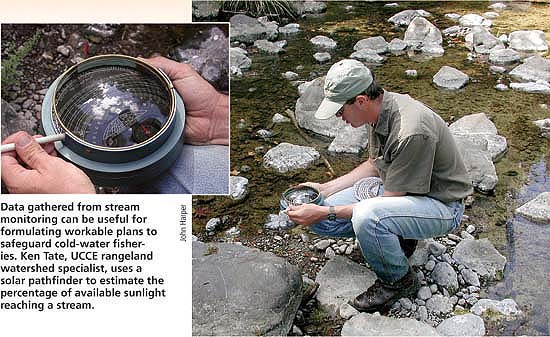
Data gathered from stream monitoring can be useful for formulating workable plans to safeguard cold-water fisheries. Ken Tate, UCCE rangeland watershed specialist, uses a solar pathfinder to estimate the percentage of available sunlight reaching a stream.
Fish responses to temperature vary by species and life stage (such as larval, fry, juvenile and adult; see page 150 )(Beschta et al. 1987; Thompson and Larsen 2004). As a result, stream-temperature criteria and objectives to safeguard cold-water fisheries habitat are often dependent upon the species occupying a particular stream reach and the life stage at which the species are present. For example, Oregon's Department of Environmental Quality established a standard of 66°F as the 7-day moving average of daily maximum stream temperature for general salmonid use, but recommends 55°F for spawning, egg incubation and fry emergence.
Glossary
Glossary: stream-temperature metrics
Daily maximum temperature: Maximum of 48 observations collected every half hour during each 24-hour day.
Daily average temperature: Average of 48 temperature observations collected every half hour during each 24-hour day.
7-day running average of daily maximum temperature: Calculated for each day as average of daily maximum temperature observed for that day and for 6 consecutive prior days.
7-day running average of daily average temperature: Calculated for each day as average of daily average temperature observed for that day and for 6 consecutive prior days.
Maximum weekly maximum temperature: Maximum 7-day running average of daily maximum temperatures observed during a period of interest (such as a specific month or critical fish life stage).
Maximum weekly average temperature: Maximum 7-day running average of daily average temperatures observed during a period of interest.
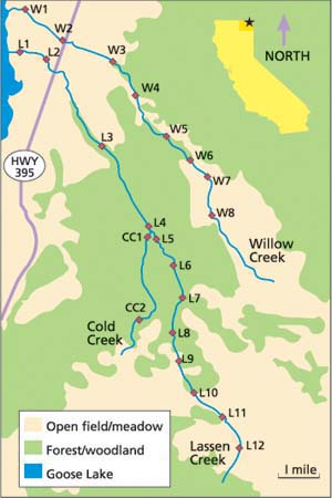
Fig. 1. Stream-temperature monitoring locations on Lassen, Willow and Cold creeks in northeastern Modoc County, Calif.
Monitoring and data collection are frequently undertaken in streams across California and the western United States. The objectives often include: (1) the evaluation of compliance with specific stream-temperature criteria; (2) the determination of temperature changes above and below a land-use activity, through a given property or stream reach, or along an entire stream network; and (3) the examination of watershed-specific associations between stream temperature and factors such as air temperature, stream flow and riparian canopy cover. Several publications provide guidance on how to plan and implement water-quality and stream-temperature monitoring (ODF 1994; MacDonald et al. 1991; US EPA 1997), but few provide guidance on how to analyze and interpret the resulting data.
While the availability of inexpensive, automatic temperature recorders has facilitated data collection, in our experience the sheer volume of data gathered often overwhelms individuals, watershed groups and agencies. As a result, the data is often not analyzed. We have also observed that when groups collect stream-temperature data, they often neglect to collect data on associated factors (such as air temperature, stream flow, canopy cover and reach length) that are required to fully interpret the stream-temperature data, in order to reach defensible conclusions for management, restoration and regulatory decisions.
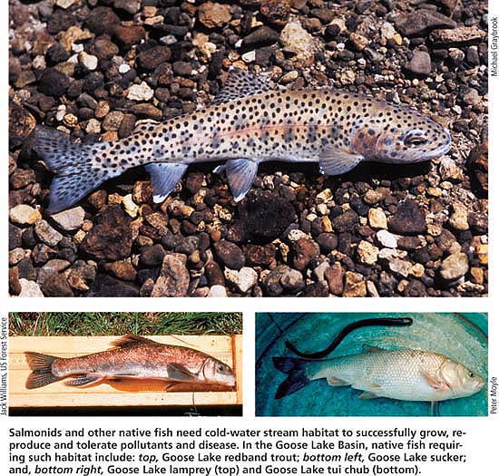
Salmonids and other native fish need cold-water stream habitat to successfully grow, reproduce and tolerate pollutants and disease. In the Goose Lake Basin, native fish requiring such habitat include: top, Goose Lake redband trout; bottom left, Goose Lake sucker; and, bottom right, Goose Lake lamprey (top) and Goose Lake tui chub (bottom).
The objective of our study was to demonstrate methods for the graphical display and analysis of the kind of stream-temperature data typically collected in monitoring efforts. We illustrate presentation formats and non-statistical approaches to facilitate the synthesis and interpretation of data for the purposes of monitoring compliance and evaluating the impacts of land-use activities. In the paper that follows ( see page 161 ), we illustrate a statistical approach to analyzing complex sets of stream-temperature data and associated parameters. For both papers, we utilize the same data set, collected during the summers of 1999, 2000 and 2001 across the Lassen and Willow creek watersheds in northeastern Modoc County (in the northeastern-most corner of California).
Lassen and Willow creek watersheds
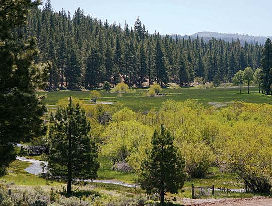
Located on the western slope of the Warner Mountains, the Lassen and Willow Creek watersheds lie parallel to each other, have a northwest aspect and flow directly into Goose Lake, which is at 4,700 feet (fig. 1). The upper reaches of both watersheds are in the Modoc National Forest and extend as high as 6,000 to 7,500 feet. Both streams flow out of predominantly publicly owned (U.S. Forest Service) mountains and into predominantly privately owned valleys and plains above Goose Lake. The public lands are managed for multiple uses including extensive livestock grazing and dispersed recreation. The private lands are used primarily for livestock grazing, as well as irrigated and dryland hay production. We selected these watersheds for study due to the willingness of landowners to cooperate, as well as in response to requests for stream-temperature information driven by local concerns for native fishes that use these streams for spawning and rearing habitat.
Although both streams reach peak runoff with snowmelt in the spring (May through June), they are primarily spring-fed during the summertime base flow (between rain-storm events, before and after snowmelt). Lassen Creek is about 14 miles long and Willow Creek is about 11 miles long. The streams are similar, but do have some clear differences. In Lassen Creek, perennial stream flow begins at about 6,000 feet and the stream stair-steps its way down through a series of small mountain meadows and steep canyons on its way to Goose Lake. In addition, Lassen Creek has one perennial tributary, Cold Creek (fig. 1). In Willow Creek, perennial stream flow begins at about 5,200 feet and the stream meanders through two relatively large open valleys connected by a canyon reach. As is typical of most mountain streams in Northern California, Lassen and Willow creeks provide cold-water habitat for trout, as well as other native fish and invertebrates. Four of these native fish species occur only in the Goose Lake basin: the Goose Lake redband trout (Oncorynchus mykiss), Goose Lake sucker (Catostomus occidentalis lacusauserinus), Goose Lake tui chub (Gila bicolor thalassina) and the Goose Lake lamprey (Lampetra tridentata). These species spend much of their adult lives in Goose Lake, but depend on Lassen and Willow creeks for annual spawning and rearing habitat, as well as for emergency refuges during prolonged drought when Goose Lake goes dry. Our group initiated stream-temperature monitoring in conjunction with the Goose Lake Fishes Working Group (a multiagency stakeholder group) in the late 1990s, due to the proposed listing of all four species under the federal Endangered Species Act. Elevated stream temperature was proposed as one of the main factors impairing habitat in both streams.

The researchers collected data in watersheds feeding Goose Lake, above; the outlets of Lassen and Willow creeks are located on the peninsula in the center. Right, Shannon Cler, UC Davis postgraduate researcher, uses a velocity meter to estimate stream flow.
Monitoring protocols
Stream-temperature data was collected from June through September in 1999, 2000 and 2001 across Willow, Lassen and Cold creeks (fig. 1). We identified the monitoring locations in 1997 and 1998 by combining field surveys of each stream with preliminary stream-temperature data collection. Monitoring locations were selected to: (1) systematically track temperature changes from the upper to lower extent of each stream; (2) dissect each stream into discrete reaches based upon changes in stream morphology and gradient, vegetative community and canopy, aspect and land management; and (3) account for the confluence of tributaries and springs within each stream channel.
At each monitoring location, stream temperature was recorded every half hour using commercially available automatic recorders (Optic Stow Away, Onset Computer Corporation). Data collection at the half-hour time-step allows for the capture of daily maximum and minimum temperatures, as well as the calculation of daily average temperature (48 readings per day), 7-day running average of daily maximum temperature, and other metrics of interest (). Here we only report the daily average stream temperature and the 7-day running average of daily average temperature. Recorders at all locations were set to take readings simultaneously on the hour and half hour (1:00, 1:30, 2:00, and so on). Temperature recorders were submerged at the bottom of the stream in areas of thorough mixing (riffles or runs) and held in place with a weight. Their depth ranged from 6 to 16 inches due to declining water levels as the season progressed, and variability in stream size and morphology (narrow and deep versus wide and shallow shape) among monitoring locations.
In order to interpret the stream-temperature data relative to environmental conditions and land-use management, we collected additional data on several associated factors. Air temperature was measured at both the lower and upper reaches of each stream (fig. 1; L1, L10, W1, W8) and recorded every half hour with automatic recorders (Optic Stow Away, Onset Computer Corporation) suspended 6 feet above the ground surface, out of direct sunlight and in areas of adequate air mixing. Stream flow was measured in late May, late July and late September each year at every monitoring location. Instantaneous stream flow was measured by hand as cubic feet per second (cfs) using the area velocity method (stream width in feet times average stream depth in feet times average stream velocity in feet per second). Stream velocity was measured with a hand-held velocity meter at the same times as water width and depth.

Fig. 2. Daily average and 7-day running average of daily average stream temperature observed at sampling locations, representing the longitudinal profile of Lassen Creek for 1999, 2000 and 2001.
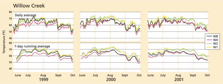
Fig. 3. Daily average and 7-day running average of daily average stream temperature observed at sampling locations, representing the longitudinal profile of Willow Creek for 1999, 2000 and 2001.

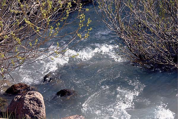
Stream flow is an important factor determining stream temperature, with daily maximum temperatures decreasing as flow increases. Facing page, left, flatter meadows, such as in the Lassen Creek watershed, slow down flow and allow warming; facing page, right, narrow canyon reaches provide natural shade and potentially force the emergence of cool subsurface stream flow. Snowpack in the Warner Mountains, above, feeds Lassen and Willow creeks in the northern range and the Pit River in the southern range (shown).
Canopy cover and solar input were measured in July 2000 at five sample locations equally spaced along the 1,000-foot stream reach immediately upstream of each monitoring location. Canopy cover — the percentage of sky blocked by vegetation — was measured with a densiometer. Solar input — the percentage of available solar input reaching the stream surface — was measured using a solar pathfinder. Canopy cover at each location was calculated from four densiometer readings taken in the middle of the stream at each location (facing upstream, left bank, downstream, right bank) following California Department of Fish and Game protocol (DFG 1998). Solar input was measured at the same locations as canopy cover with the solar pathfinder held just above the stream surface in the middle of the stream, following standard methods (Platts et al. 1987). The design of the solar pathfinder allows for calculation of monthly solar input from a single reading. Solar input readings are correlated to the vegetative canopy readings but are also affected by stream aspect and topographic features such as canyon walls or nearby mountains, which may block the sun during portions of the day or year.
Temperatures along streams
Monitoring groups are often interested in comparing stream temperature at specific locations along a stream, for example, on a specific reach (such as L12 versus L10) or along a longitudinal profile from upper to lower stream locations (such as L12 versus L11 versus L10)(fig. 1). This information can be used to identify and prioritize points of concern for fisheries (such as areas exceeding temperature standards), restoration opportunities (such as riparian planting to increase canopy cover) or land-use activities that should be mitigated (such as excessive warm irrigation-water returns).
One way to display and analyze data from monitoring locations along a stream system is to plot temperature at multiple locations over time on the same graph. Figures 2 and 3 synthesize a cumbersome raw data set of 158,112 data points (nine locations, times 3 years, times 122 days per year per location, times 48 readings per day), yet still reveal seasonal trends (such as peak temperatures in August and rapid reduction during the first week of September) that would be lost in monthly, seasonal or annual statistics (such as average and maximum). These figures provide a simple means of illustrating which stream was warmer or colder, and how stream temperature changed through the summer and across years, as well as an initial assessment of how stream temperature changed over time along a given stream reach or system.
For example, we found that Willow Creek was consistently warmer than Lassen Creek, which means that Lassen Creek provided more cold-water habitat than Willow Creek (figs. 2 and 3). Mean stream temperature from the top to bottom of Lassen Creek could increase from 10°F to 20°F on a given day (L12 versus L2), with the greatest increase in temperature occurring on a reach flowing through a naturally open meadow (between L12 and L10). Willow Creek, on the other hand, cooled as it flowed through a long, shaded canyon reach (between W8 and W4) and then increased in temperature as it continued downstream. The reduction in stream temperature between locations W8 and W4 on Willow Creek varied by year. Cooling through this reach was greatest in 1999, which had higher stream flows than 2000 and 2001, both years of regional drought and low flow.
For simplicity and clarity, the statistics that best reveal the area of concern should be plotted. The 7-day running average results in a smoother plot that facilitates comparisons among multiple locations. By contrast, if the concern is the acute effects of daily temperature variations, then plotting the daily average or maximum for only one or two sites is more clear and informative.
Comparisons between stream reaches
While graphics such as figures 2 and 3 allow for the efficient display and initial interpretation of the large, raw data sets typically collected by stream-temperature monitoring efforts, additional data reduction and graphical analysis are required to compare the change in stream temperature occurring between different reaches. With limited budgets for restoration efforts (such as riparian planting), reach-specific information on rates of temperature change can facilitate the optimal allocation of restoration resources to stream reaches within the watershed.
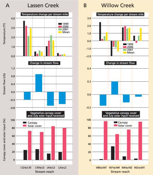
Fig. 4. For reaches of (A) Lassen Creek and (B) Willow Creek: (top) change in daily average stream temperature (°F) from June through September per stream mile for 1999, 2000 and 2001, including the average (mean) for 1999, 2000 and 2001; (middle) average change in stream flow in cubic feet per second (cfs) measured during August 2001; and (bottom) percentage vegetative canopy cover and percentage of available solar input in July.
On Cold Creek, willows budding in early spring will provide shade to reduce stream-temperature gains in the summer.
As in most monitoring efforts, the locations on Lassen and Willow creeks were selected to isolate reaches based upon changes in factors such as geomorphology, vegetation and flow, which are primary environmental variables that interact with land use to determine stream temperature. This approach is important to insure that the data collected relates spatially to important core watershed characteristics, land uses and the habitat available to resident fish. As a result, the distance between monitoring locations, and thus stream reach length, varies (fig. 1). Reach length confounds the direct interpretation of stream-temperature changes (figs. 2 and 3). One would expect greater overall change in temperature across longer reaches than across shorter ones. As such, the direct comparison of stream-temperature change through reaches of different lengths requires standardization for reach length.
An efficient and simple approach to account for reach length is to divide the change in temperature through each reach by the length. The resulting unit is “change in temperature per stream mile” (or unit length). To illustrate this approach, we examined the change in daily average stream temperature during the summer (June through September) across four reaches of Lassen and Willow creeks (figs. 4A and 4B [top]). We took the average of the differences in daily average temperature between two monitoring locations (such as L12 and L10) for the summers of 1999, 2000 and 2001, then divided this average by the distance between the two locations. Depending upon the specific interest of the monitoring group, similar calculations could be generated and graphed on a daily, weekly or monthly basis, using average, maximum or minimum temperatures.
Figures 4A and 4B (top) provide directly interpretable information for managers, groups and other interested parties working on watersheds. For example, they clearly identify stream reaches within each watershed with the highest gains in temperature per stream mile. In Lassen Creek, the rate of warming was far greater in the reaches between L12 and L10 and between L4 to L3 than other reaches. In Willow Creek, the rate of temperature increase was consistently highest in the reach between W4 and W2. Although Willow Creek is warmer (figs. 2 and 3), the rate of heating across Lassen Creek was consistently greater. It is conceivable that the background, or natural, temperature of Willow Creek is greater than that of Lassen Creek, perhaps because perennial flow starts at a lower elevation in Willow Creek and flows through two large open meadows, while Lassen Creek flows through more-forested canyons.
Although both Lassen and Willow creeks gained heat through their lower reaches, which are associated with irrigation-water diversion and return, these lower reaches were not the sections of either creek with the highest temperature gains. This does not imply that irrigation management does not influence stream temperature, but rather that temperature gains in the middle and upper reaches must also be considered if reduced temperatures in the lower reaches are a habitat objective. These graphs do not establish cause and effect; rather, they facilitate understanding of watershed-scale temperature dynamics and serve as an effective assessment tool.
Temperature and associated factors
The collection of data on factors that may affect stream temperature is the first step in translating speculation into defensible conclusions. It is difficult to use graphical analysis for evaluating the simultaneous and interacting relationships that might exist between stream temperature and associated factors such as air temperature, stream flow and riparian canopy. However, graphical analysis can provide useful insights for improving local monitoring schemes and more thoroughly quantifying statistical relationships. To illustrate this point, we display data on the change in stream flow as well as riparian canopy and solar input (fig. 4).
Comparison of figures 4A and 4B (middle) indicates that temperatures rose in all Willow Creek reaches that lost stream flow (that is, less water emerged from the reach than entered it), while the temperature dropped in the reach that gained stream flow (W7 to W4). This reach is situated in a bedrock canyon below a meadow reach. It is likely that stream flow lost to the channel's subsurface zone (the gravels and sediments in and under the channel bed) in the reach immediately upstream (W8 to W7) was forced up by bedrock to re-emerge as surface flow in the reach from W7 to W4. In addition, this area of the watershed has multiple diffuse seeps and springs along the stream channel. Regardless of the source of the increased subsurface flow, it is likely that it would be cooler (about 50°F to 55°F) than surface water in the stream (Stringham et al. 1998). Similarly, on Lassen Creek the reach from L10 to L5 gained stream flow and had relatively low rates of temperature gain.
Following a graphical approach that only considers a single associated variable (univariate), one might conclude that flow is the main factor influencing the direction and rate of temperature change, because stream reaches that lost

Stream cover is provided by trees and shrubs such as, top, conifers and aspens, and, above, willows.
This graphical comparison indicates that there are probably strong relationships between the factors considered. However, it is inappropriate and likely misleading to use a univariate, graphical analysis approach to (1) fully explore and quantify these relationships, (2) determine if stream flow and canopy interact to influence stream temperature, or (3) determine if the influence of canopy or stream flow is different between streams. Answering these complex monitoring questions requires a multivariate statistical analysis of a data set containing stream temperature and associated factors ( see page 161 ). Fortunately, relatively simply collected data sets can be subjected to appropriate graphical and statistical analyses.
Data helps prioritize resources
We have demonstrated a graphical display and analysis approach by which data collected in typical stream-temperature monitoring projects can be interpreted by and presented to land managers, watershed groups and other interested parties. This approach is simple and nonstatistical, facilitating timely local analysis to achieve monitoring objectives such as evaluating stream temperature across a watershed for comparison to temperature criteria, and identifying watershed areas with high or low rates of stream-temperature gain. This level of analysis can translate large raw data sets into information that local managers and water-resources agencies can use to identify and prioritize the allocation of limited restoration and management resources.
In order for stream-temperature data to be useful, related data such as stream canopy, air temperature and stream flow should be collected. In mid-Lassen Creek, shade is naturally low, and willows serve as the primary source of vegetative cover.
Graphical analysis facilitates evaluation of stream-temperature monitoring data