


All Issues
Weeds accurately mapped using DGPS and ground-based vision identification
Publication Information
California Agriculture 58(4):218-221. https://doi.org/10.3733/ca.v058n04p218
Published October 01, 2004
PDF | Citation | Permissions
Abstract
We describe a method for locating and identifying weeds, using cotton as the example crop. The system used a digital video camera for capturing images along the crop seedline while simultaneously capturing data from a global positioning system (GPS) receiver. Image time-stamps were synchronized with GPS time so that GPS coordinates could be overlaid onto selected images. The video system continuously mapped nutsedge weeds and crop plants within the seedline, allowing weed locations to be described with centimeter-scale accuracy when using a real-time kinematic GPS (RTK-GPS). This system may be used to develop maps of weed and crop populations as part of precision crop-management decisions.
Full text
Knowing where recurrent weeds or insect infestations occur over multiple growing seasons can facilitate the selective application of herbicides, pesticides and soil treatments. This information can be economically beneficial to growers because it allows areas at high risk for weed infestation to be treated prior to weed emergence while areas below an economic threshold can remain untreated. There is an ongoing need to reduce chemical applications, due to continued concern among regulators and economic constraints on growers. The methods described in this report are one step in that direction.
A large amount of research has been conducted on remote sensing with aerial and satellite imagery for yield and weed mapping in agriculture. GIS/ ArcView/ArcInfo systems continue to be widely used for decision-making in precision agriculture and crop management. In-field vision detection (a nondestructive measurement) for site-specific crop management has a higher resolution (“centimeter scale” accuracy) than satellite or aerial imagery, which typically have 3.28-foot to 32.8-foot (1-meter to 10-meter) scale accuracy. In-field vision systems may also allow descriptions of weed species.

Fig. 1. Toolbar-mounted weed-mapping and location system. A tractor-mounted toolbar with a camera enclosure and GPS antenna were used to acquire images and location data.
Discrete sampling has been the most common method to identify and map weeds but it is time consuming and small grid sizes are not feasible for mapping large areas (Rew and Cousens 2001). Furthermore, quadrant size and sampling intensity are totally arbitrary, and large areas of the field can remain unsampled.
Manual surveys of weed locations in fields were described by Webster and Cardina (1997), who mapped and assessed accuracy in simulated weed patches of 16.4, 164.1 and 1,641 square feet (5,50 and 500 square meters) using a backpack fitted with a global positioning system (GPS) receiver and antennae. Errors associated with area measurements were lowest with the 1,641-square-foot (500-square-meter) area (3% to 6%) and largest in the 16.4-square-foot (5-square-meter) area (14% to 32%). The authors estimated that the 25 weed patches with the largest areas would require 21 minutes of continuous data collection (probably not including post-processing time for management decisions). Navigation assessments upon returning to previously mapped locations indicated that 27% of the original quadrants were found, and of those, 73% were found within 3 feet (1 meter) of the original location.
Van Wychen et al. (2002) discussed a continuous mapping system using an all-terrain vehicle mounted with a differential GPS receiver (DGPS), computer and human crop consultant. Maps were created by traversing the perimeter of patches, and transects across the field were driven every 30.2 feet (9.2 meters). The discrete method of developing a wild-oat seedling map entailed walking parallel transects in specified grid patterns and counting wild-oat density in 3.1-square-foot (0.29-square-meter) rectangular grids and georeference locations with a GPS receiver and computer. The results found that continuously sampled weed-seedling maps with weeds identified as present or absent were cost effective if the accuracy in locating patches was greater than 70%.
Manh et al. (2001) indicated that weed identification continues to be difficult due to the complexity of ambient outside light and variability in plant morphology (form and structure). Their research described weed leaf segmentation (the identification of individual leaves) using deformable templates (a machine-vision technique where the leaf pattern or template is modified or deformed to match the unique shape of a specific leaf). The approach applied prior knowledge to the object searched and improved the weed segmentation stage. Although the study considered only one weed species, partially occluded (hidden) leaves were identified correctly. Additional work by Tang et al. (2001) described a sensor-based, high-resolution, realtime system for mapping in-field variability in weed load. Cameras were suspended (without shading) 10.5 feet (3.2 meters) above the soil surface, but results found that variability in outdoor lighting resulted in variations in camera performance.
Research at UC Davis developed a weed-control system for selective herbicide applications using machine vision (Lee et al. 1999). The system was towed by a tractor traveling 0.75 miles per hour (mph; 1.2 kilometers per hour) and was able to process images within 0.344 seconds. In field tests 24.2% of tomatoes were incorrectly categorized as weeds and sprayed, while 52.4% of weeds were not sprayed. Lamm et al. (2002) continued this work in cotton and developed a nonmorphological machine-vision technique that could discriminate between partially occluded narrow-leaf and broadleaf plants. The system identified and sprayed 88.8% of the weeds during in-row seedline image capture and analysis; these results are comparable to hand-hoeing, which eliminates only 65% to 85% of weeds.
The machine-vision systems described in the previous studies may be prohibitively expensive if used for large-scale weed mapping or in conjunction with robotic spraying. In a recent study, Gliever and Slaughter (2001) developed a cost-effective method for successfully identifying and mapping weeds within crops. The software used an artificial neural network with a demonstrated accuracy of 92% for weed recognition.
Research on discriminating between weeds and crops under ambient light conditions continues to be a challenge. Recent work at UC Davis resulted in a mapping system that can be used to identify weed densities at specific geographic locations. The system links GPS coordinates to images of the crop seedline for future management analysis and decision-making. This type of mapping system can be a feature in current software used in precision agriculture. Automated GPS mapping of images linked to latitude and longitude is a new method for inspecting remote areas for weed and insect problems during the early stage of crop growth.
The objective of this study was to acquire GPS coordinates simultaneously with digital images of weeds in early-season cotton and to develop an automated routine to identify and map weed and crop densities for crop management.
Weed mapping in a cotton field
The crop rotation schedule in the test field prevented multiyear data collection for this study. Multiyear images of the same fields would allow for verification of returning or localized weed infestations. Although this was not possible, the system design and concept for future software use are still valid. Data from 2002 is used here to show proof of the concept.
The test site was on a commercial farm in the San Joaquin Valley, outside of Corcoran. Cotton was planted in April 2002. Images of early-season cotton were acquired approximately 10 days after planting. Yellow nutsedge (Cyperus esculentus L.) was the only weed species present in the test site. Two test plots (S3 and R14) were studied. The S3 test plot was 0.74 acre (0.3 hectare) with approximately 280-foot (85-meter) row lengths and 18 rows on 3.3-foot (1-meter) spacings; the R14 test plot was 0.35 acre (0.14 hectare) with 150-foot (45-meter) row lengths and 17 rows on 3.3-foot (1-meter) spacings. Rows for both test plots were aligned on an ENE-WSW line. These plots were selected because these fields had a history of patchy weed populations with weed-free areas, as well as areas with a high percentage of weed cover.
The GPS antenna was located along the optical axis of the digital camera mounted on a tractor-drawn toolbar (Model DCR-TRV900,3 CCD, Sony). The camera was set inside a sheet-metal enclosure that prevented sunlight from entering the image acquisition area, and diffuse artificial lighting was provided (Lamm et al. 2002). The camera viewed a 6-inch-by-4-inch region along the seedline and was equipped with removable digital videotape (miniDV format, 60-minute capacity). Continuous digital video of the seedline was collected in the camera's progressive scan mode to allow the full vertical resolution to be utilized while collecting images from a moving vehicle. Field location (latitude and longitude) and ground speed of the vehicle were monitored using a CASE AFS Universal Receiver (Model SB2400 with fast update option, DGPS U.S. Coast Guard beacon signal and NMEA-0183 data output strings) interfaced with a portable computer (Inspiron 3800/Celeron 500, Dell Computer) for GPS data storage. Data was captured from the GPS receiver at 10 Hz via an RS-232 serial line.
Video and coordinate data were simultaneously collected while traveling along the seedline of the crop at an average speed of 1.57 mph. GPS time was synchronized with the digital videotape time-code by filming GPS time on the receiver display at the beginning of each row. The NMEA-0183 GPS data string was post-processed; latitude and longitude were transformed to x, y and z metric coordinates using the coordinate conversion equations presented by Dana (1999) for distance traveled. The coordinate data was processed for each approximately 1.64 feet (0.5 meters) of forward travel and the corresponding time-stamps (from the NMEA-0183 data string) annotated for that travel distance. This data was used to overlay coordinates on each video frame representing 1.64 feet (0.5 meters) of forward travel. By counting through the frames based on GPS time downloaded from the GPS receiver, the video frame for each GPS coordinate could be identified.
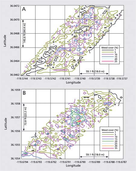
Fig. 2. Percentage weed-cover contour map of plots (A) S3 and (B) R14, developed by the automated location and identification process. Source: (Downey et al. 2003.
Digital video was transferred from tape and stored in AVI digital video format on the computer hard disk using Adobe Premiere (v. 6, Adobe Systems) software and an IEEE-1394 communication line. A Visual C++ (v. 6.0, Microsoft) program was used to extract the video frame corresponding to each GPS coordinate and to label each image with its GPS coordinate. A total of 4,962 video frames (3,366 for S3 and 1,596 for R14) were extracted from the two test plots. An additional C++ program was used to automatically inspect each image for the presence of cotton and nutsedge plants using Gliever and Slaughter's (2001) method, in which the image is subdivided into 128 grid cells, each corresponding to a 0.2-square-inch (1.2-square-centimeter) region of the seedline.
The percentage weed cover or cotton density at each GPS coordinate was defined as the percentage of grid cells containing nutsedge or cotton leaves, respectively, in the corresponding image. Cells that contained both cotton and nutsedge leaves were classified as cotton. Fifty video frames were randomly selected for manual validation of the accuracy of the image processing method. A percentage weed-cover or cotton-density contour map was produced for each plot using the contour procedure in commercial software (SAS/GRAPH, SAS Institute, 1999).
Weed map verification
The mean percentage of nutsedge cover, or number of grid cells in which nutsedge leaves occurred was 5.8% and 8.0% in the S3 and R14 plots, respectively, with standard deviations of 5.5% and 6.0% (fig. 2). These maps show the variability in percentage weed cover across the plots with patches of high weed densities observed toward the centers of both. The 4,962 images analyzed to produce these maps represent a total land area of 800 square feet (74.4 square meters) distributed over 1.64-foot (0.5 meter) intervals along the seedlines in 1.1 acre (0.44 hectare) of a commercial cotton farm.
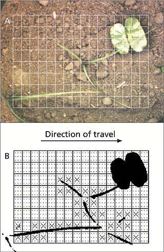
Fig. 3. (A) A cotton plant partially occluded by a nutsedge leaf; (B) weed map of (A) where grid cells containing nutsedge leaves are marked with an “X.” Note: A thin piece of crop residue was mistakenly mapped as a weed due to an error in the color classifier. Source: (Lamm 2000.
Seventy-four percent of the 221 nutsedge leaves present in the 50 validation images were correctly identified. The primary causes of misclassification of nutsedge leaves (as cotton) were occlusion and the decision to classify grid cells containing both nutsedge and cotton as cotton (fig. 3). The original purpose of the weed-map algorithm developed by Gliever and Slaughter (2001) was to create a precision spray map. In this application, grid cells containing both cotton and weed leaves were mapped as cotton in order to avoid spraying the cotton plants. The secondary cause of misclassifying nutsedge as soil was the low resolution of sampling points (12 points per 0.2-square-inch [1.2-square-centimeter] grid cell) in the image, which caused small, thin leaves to be missed. These results are slightly lower than the weed recognition rate observed by Gliever and Slaughter (2001) or Lamm et al. (2002).
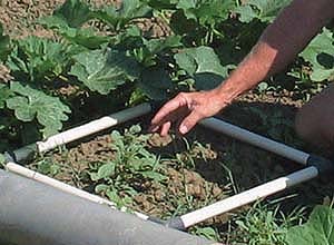
A weed scientist manually counts weeds inside a frame. Weed mapping using machine vision and a global positioning system is much faster and just as accurate.
Ninety-two percent of the cotton leaves present in the 50 validation images were correctly identified. The primary cause for misclassifying cotton leaves as weeds or soil was brown tissue damage on the leaf. Brown spots on a leaf were classified as soil, and depending upon the quantity and size of the spots, the resulting visual pattern was frequently classified as a weed. These results are comparable to those observed by Gliever and Slaughter (2001) and better than those observed by Lamm et al. (2002). The overall accuracy of the system was about 85%, which was comparable to that observed by Lamm et al. (2002) and similar to the 65% to 85% accuracy of a typical handhoeing crew (Vargas et al. 1996).
When implemented on a computer with a 1.7 GHz processor (Intel Pentium 4), the weed-map algorithm developed by Gliever and Slaughter (2001) could map the weeds in a 320 x 240 pixel image at a rate of 10 frames per second. While the post-processing of the GPS data and the conversion of the digital video to a format accessible to the image processor required manual intervention, the creation of the weed maps themselves was completely automated. This represents a dramatic labor savings when compared to traditional methods of weed mapping. In addition, the manual tasks are primarily associated with the initial setup and are not dependent upon the number of images analyzed. An automated system of this type can provide a significantly more detailed description of the percentage weed cover in a field. In this study, the images were sampled every 1.64 feet (0.5 meters) of seedline due to the accuracy of the DGPS system. However, the system is capable of analyzing every frame and making a continuous map of the entire field.
While this paper focused on weed mapping, the system could easily produce a map of crop density at the same time. The weed and crop maps could be utilized as layers in a GIS database and incorporated in a comprehensive assessment of crop yield, and to develop site-specific input application maps.
Mapping as accurate as hoeing
An automatic weed-mapping location and identification system was developed and tested in a commercial cotton field. The system used a video camera, image-processing system and DGPS data-logger to map nutsedge in cotton. The system had an overall accuracy of about 85%, similar to the weed-control accuracy of a typical hand-hoeing crew.
The system demonstrates the technical feasibility of automated weedmapping. With a processing rate of 10 images per second, the potential for labor savings compared with conventional weed-mapping methods is significant. The technique could be combined with farming operations — including planting, cultivating or chemical applications (such as fertilization or insecticide sprays) — further reducing labor, fuel and equipment (such as tractor) costs. An automated, low-cost, weed mapping system would allow growers to track weeds throughout the season to provide feedback on the efficacy of weed management programs and in GPS yield map analysis. The authors acknowledge that the current economic cost of computer vision equipment and practical feasibility of using video cameras in ground-based agricultural field operations continues to be a challenge for future implementation. Also, future research is needed to expand the scope of weed identification algorithms, for example to distinguish differences between broadleaf weeds and broadleaf crops, in addition to a wider range of weed species.
Weeds accurately mapped using DGPS and ground-based vision identification