


All Issues
New crop coefficients estimate water use of vegetables, row crops
Publication Information
California Agriculture 52(1):16-21. https://doi.org/10.3733/ca.v052n01p16
Published January 01, 1998
PDF | Citation | Permissions
Abstract
To estimate the water use of vegetable and row crops, crop coefficients were developed using portable Bowen ratio instruments that were constructed and tested against lysimeters. These instruments measured evapotranspiration (ET) in fields of vegetable and row crops at various developmental stages. The crop coefficient was calculated at different percentages of ground cover using a direct ratio between the ET of the crop and that of a reference grass, which was calculated using meteorological data calculated from local CIMIS weather stations. The crop coefficients for most of the crops increased as the percentage of ground cover increased.
Full text
By more accurately estimating the amount of water crops use, growers can save water by applying only as much water as needed.
In a typical nondrought year, agriculture in California uses approximately 75% of the state's developed water supply. In 1990, the state Department of Water Resources (DWR) estimated that California farmers used 27 million acre-feet of water. This is equivalent to a 30-foot-by-30-foot column of water that extends all the way to the moon.
Crops unavoidably use large quantities of water. More than 98% of the water absorbed by the roots of irrigated crops is transpired as water vapor to the atmosphere over the course of the season. Most of this water is lost through stomata, specialized pores on leaf surfaces that allow water vapor to exit the leaf and allow carbon dioxide, which is necessary for photosynthesis, to enter. Therefore any measures to reduce water loss through stomata, specialized pores on leaf surfaces that allow water vapor to exit the leaf and allow carbon dioxide, which is necessary for photosynthesis, to enter. Therefore any measures to reduce water loss through the leaves (that is, to reduce transpiration) will concomitantly reduce photosynthesis and crop yields.
Because irrigated agriculture uses such a large fraction of the state's developed water supply, it is essential that water is used as wisely and efficiently as possible. The DWR is a proponent of this need and in the 1980s awarded UC a large grant to conduct research and develop information that will help growers achieve this goal. The overall project was called the California Irrigation Management Information System (CIMIS). Much of this grant was dedicated to the development of a network of weather stations that are located in various climatic regions of the state and are now operated by the DWR. These weather stations collect meteorological data and use a modified Penman formula to estimate the reference evapotranspiration (ETo) for the region associated with that station.
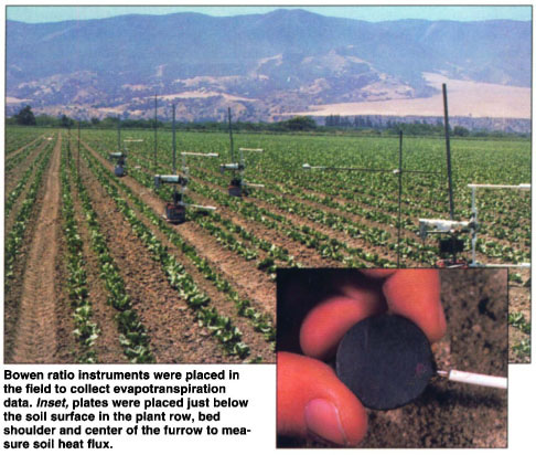
Bowen ratio instruments were placed in the field to collect evapotranspiration data. Inset, plates were placed just below the soil surface in the plant row, bed shoulder and center of the furrow to measure soil heat flux.
The ETo is the amount of water a healthy, actively growing cool-season grass subjected to those conditions uses over a specified time. The importance of this value is that crops in that region will use water in direct proportion to the evapotranspiration of this reference grass. Therefore accurate estimates of crop water use (crop evapotranspiration, ETc) depend to a large extent on the accuracy of the coefficients used to relate ETo to ETc. These coefficients are referred to as crop coefficients (Kc) and are calculated as Kc = ETc/ETo.
Our objective was to develop crop coefficients for several vegetable and row crops in California, particularly those for which reliable values were lacking. Of particular concern are Kc values for many vegetable and row crops reported in United Nations Food and Agricultural Organization Irrigation and Drainage Paper #24 (FAO 24) (Doorenbos and Pruitt 1977). To develop accurate crop coefficients, we had to develop, construct and test instruments that could measure ET in growers' fields in the vicinity of CIMIS weather stations that reported ETo values.
Measuring evapotranspiration
We selected the Bowen ratio energy-balance method for estimating ETc because it is reasonably accurate and the instruments can be made portable. Although the theory for this methodology was developed in the 1920s, no instruments were commercially available at the beginning of this project in 1986. Therefore it was necessary for scientists who wanted to use this method to design, construct and test our own instruments.
The Bowen ratio energy-balance method for the determination of crop ET is based on the principle of energy conservation and accounts for vertical energy fluxes into and out of a crop surface.
The energy balance equation is Rn = S + H + LE, where Rn is the net flux of solar radiation, S is the soil heat flux, H is the sensible heat flux and LE is the latent heat flux.
This equation states that the net flux of radiation entering the crop environment dissipates through warming of the soil, warming of the air and evaporating water. These three processes account for nearly all of the energy entering and leaving the crop environment. Other processes such as photosynthesis are assumed to be negligible, and horizontal energy inputs and outputs (that is, advection) were minimized by situating the instruments in large fields with adequate fetch upwind. Fetch is the upwind distance of the vegetation underlying the instrument.
The LE term is not measured directly, but indirectly through the calculation of the Bowen ratio (ß). The Bowen ratio is the ratio of sensible to latent heat flux (H/LE). It is proportional to the ratio of the air temperature gradient to the vapor pressure gradient over a specified vertical distance above the crop. The advantage of ß is that H and LE do not have to be measured directly, just a temperature and humidity gradient above the crop canopy. By mathematically rearranging the energy balance expression and by making some reasonable assumptions, the LE term can be calculated as LE = LE = Rn-S/ß + 1 A constant is then used to convert LE to evapotranspiration of the crop (ETc).
Design of instruments
The Bowen ratio instruments were designed to be portable so that they could be easily transported and set up in most field situations. The main portion of the instruments consists of an apparatus and sensors that measure air and dew point temperature at two points above the canopy. Details of instrument design are reported elsewhere (Grattan 1988) and are discussed here only briefly.
The distance between sampling points was fixed at 3 feet (0.9 m), but the upper and lower sampling points could be adjusted up or down to accommodate different crops or crops at different heights. Normally the lower arm would be adjusted to about 6 inches (15 cm) above the canopy.
Air temperature was measured using platinum resistance temperature sensors placed approximately 1 inch from the opening of each air-intake arm. Mylar-coated heat shields were suspended over the portion of the PVC pipe where the temperature sensors were located. The dew point temperature was measured with a Dew-10 chilled mirror hygrometer. Air intake and purge fans draw air in from either the upper or lower intake arm, depending on the position of the switching-valve assembly. Continuous airflow prevented heat buildup in the air intake arms, allowing for accurate air temperature measurements. Because dew point temperature depends on only vapor pressure and atmospheric pressure, temperature changes in the air traveling to the hygrometer have no effect on the dew point measurements. Measurements were taken every 2 minutes over the day from either the upper or lower sampling position, and data were stored in a datalogger.
Individual sensors were also installed to measure Rn and S. Net radiation was measured with a Fritschen type net radiometer mounted 3 to 7 feet above the canopy and 15 feet away from the main Bowen ratio apparatus to avoid interference from reflected light. Three soil heat-flux plates were placed just below the soil surface in the plant row, bed shoulder and center of the furrow, and values were averaged to determine S.
The datalogger, Bowen ratio instrument and sensors were all connected to a central control box, which was painted green to reduce additional reflective interference. Twelve-volt batteries supplied power to operate the fan, the switch-assembly motor and the Dew-10. All sensors, including the temperature sensors and Dew-10, were periodically calibrated to assure accuracy.
Instrument testing
We tested the Bowen ratio energy-balance instruments in fields with lysimeters to compare ET estimates of each. Lysimeter ET has generally been regarded as the standard against which all other measures of ET have been compared. We did most of the testing on the Davis campus using large floating and weighing lysimeters, but other tests also took place using a smaller weighing lysimeters, but other tests also took place using a smaller weighing lysimeter (that is, 11 feet2 [1 m2]) at the UC West Side Research and Extension Center near Five Points.
Davis campus comparisons were made routinely to ensure that the ET estimates from the Bowen ratio system remained accurate. In one rigorous month-long test in April, Bowen ratio instruments collected data over a full cover of barley. Kc values were determined using ET from either the Bowen ratio instrument or the lysimeter between 8 A.M. and 5 P.M. PST and CIMIS ETo during this same period. Mean Kc values and standard errors for the weighing and floating lysimeters were 1.13 + / - 0.03 and 1.24 + / - 0.04. Equivalent value using the Bowen ratio instrument was 1.18 + / - 0.02. These values are not statistically different.
Kc as function of canopy cover
The Kc values reported here are described as a function of the percent canopy that shades the ground rather than as a function of time. Most Kc values for annual crops (including those in FAO 24) are reported as a function of time after planting, which is convenient for projecting crop water needs and scheduling irrigations.
The disadvantage of describing Kc's as a function of time is that it does not take into account environmental and cultural factors that influence the rate of canopy development, Climate can have a profound influence on the rate of canopy development, particularly in the spring when temperatures for a given week often vary from year to year. Row spacing and plant density after thinning also affect the rate of canopy development. This can lead to large errors in estimating daily ET if Kc is expressed solely on days-after-planting, particularly during early times before maximum ET is achieved. Expressing Kc values as a function of canopy cover eliminates these variables.
Measurement of canopy cover
We chose a method to measure canopy cover that is relatively easy, is reproducible and can readily be done by irrigation managers. We counted the number of centimeters on a meter stick lying flat under canopy that were either shaded (ground cover < 50%) or unshaded (ground cover > 50%). Ground-cover measurements were made systematically along a transect in a representative portion of the field upwind from the instruments close to noon. At each measuring site along the transect, measurements were made perpendicular to furrows at incremental distances in between furrow centers, and values were averaged. At each times the method had to be slightly altered for a particular crop at a given developmental stage. For example, for young lettuce less than 20% ground cover, it was easier to determine the average area covered by individual plants, measure the plant density (number of plant/area) and then determine the percentage of ground cover.
We are aware of other techniques for assessing canopy cover, such as light bars and photographic methods, but our intent for this study was to provide growers with a practical method that they could readily adopt. If new, accurate methods become economically practical to the grower in the future, correlations can be made between our simple technique and these new methods.
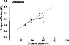
Fig. 1. Artichoke crop-coefficient functions in relation to the percentage of canopy cover that shades the ground. Dashed line Indicates Kc values estimated from FAO 24.

Fig. 2. Pinto bean crop-coefficient functions in relation to the percentage of canopy cover that shades the ground. Dashed line indicates Kc values estimated from FAO 24.

Fig. 3. Broccoli crop-coefficient functions in relation to the percentage of canopy cover that shades the ground. Dashed line indicates Kc values estimated from FAO 24.

Fig. 4. Lettuce crop-coefficient functions in relation to the percentage of canopy cover that shades the ground. Dashed line indicates Kc values estimated from FAO 24.

Fig. 5. Melon crop-coefficient functions in relation to the percentage of canopy cover that shades the ground. Dashed line indicates Kc values estimated from FAO 24.

Fig. 6. Onion crop-coefficient function in relation to the percentage of canopy cover that shades the ground. Dashed line indicates Kc values estimated from FAO 24.
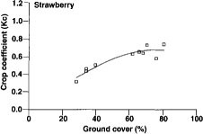
Fig. 7. Strawberry crop-coefficient functions in relation to the percentage of canopy cover that shades the ground. FAO 24 does not provide Kc values for strawberries.
Instrument placement
UC farm advisors in the different regions identified growers who had fields that suited our needs and who were willing to cooperate. Each selected field had sufficient fetch (> 300 feet) upwind from the instruments, and crops in the field appeared uniform, healthy and free from obvious disease, water or salt stresses. Fields were furrow irrigated after seeding establishment. The only exception was strawberries, which were drip irrigated under a plastic much.
In fields with less than 100% cover, data were collected only when the exposed soil surface appeared dry. This was done to avoid large variability in Kc measurements that would occur if measurements were done regardless of soil surface conditions. We had as many as five Bowen ratio instruments operational at one time. At times we took replicate measurements in the same field, while at other times we took measurements in different fields planted to the same crop but at different percent canopy covers.
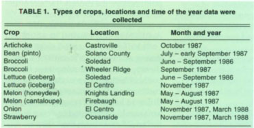
Data were collected over crops planted in different parts of the state (table 1). We found no difference in data for a particular crop collected in different regions of the state, so we combined the data and constructed Kc functions on a crop-by-crop basis. It is important to note that this should not be taken as a given for all crops in all locations, because a change in climate, such as temperature, humidity or wind speed, may not influence the ET rate of the crop and reference grass proportionally.
Honeydew melons are vegetatively more vigorous than cantaloupe (var. PMR-45) and are faster to achieve full cover. Nevertheless, there was no distinction between melon types when Kc's were expressed as percent cover, so data in this case were also combined.
Crop coefficients
The relationships between canopy cover and crop coefficient for the various crop are shown in figures 1 through 7. Each data point represents a daily average for a given instrument placed in a particular field. Each daily point was calculated by summing up hourly crop ET estimate from the Bowen ratio system and dividing that by the sum of the ETo estimates provided by the local CIMIS weather station for the same daylight hours that the instruments was collecting data in the field.
The dashed lines in figures 1 through 7 are Kc values that were estimated using information from FAO 24. They assume that the Kc values increase linearly as a function of time between 10% and about 75% ground cover. Because the percentage of ground cover increases in an approximately linear fashion during rapid growth, we assumed that the Kc values increase linearly as a function of coverage during the rapid growth period. FAO 24 assumes that there is no further increase in Kc after the crop finishes rapid growth, so the Kc values do not increase above 75% ground cover in figures 1 through 7. The Kc value at 10% ground cover was found by iterating the Kc values until the resulting line appears to match the observed data. It was not possible to determine the Kc at 10% ground cover using the method described in FAO 24 because the irrigation and rainfall frequency greatly affect Kc values during the initial growth period.
Our results indicate that the crop coefficients change as a quadratic function of percentage ground cover for most of the crops that achieve full cover (100% ground cover). We there-fore used quadratic expressions to fit the data from all of the crops.
Artichoke
Crop coefficient values were determined for artichokes in fields near Castroville that ranged in canopy cover from 28% to 60% (fig. 1). The curve was forced through the origin because the range in percent of ground cover was small and the unadjusted curve produced a negative value at 0% ground cover. The polynomial expression is
Kc = -0.000165G2 + 0.021G; r2 = 0.60
Kc and G refer to the decimal crop coefficient and percent of ground cover, respectively. Our Kc values were less than that predicted by FAO.
Bean (pinto)
Kc values for pinto bean were determined in a field near UC Davis from late July to early September, corresponding to a change in canopy cover from 13% to 85% (fig. 2). The polynomial expression that fits the data is
Kc = -0.000105G2 + 0.016G + 0.33; r2 = 0.69
Our Kc values agree fairly well with the FAO numbers up to about 60% ground cover. Thereafter our values were less than those estimated by FAO.
Broccoli
Kc values for broccoli were determined in fields in both Soledad and Wheeler Ridge in Kern County were the canopy cover increased from 17% to 100% (fig. 3). The polynomial expression is
Kc = -0.000009G2 + 0.0093G + 0.17; r2 = 0.74
Our Kc values were slightly less than that estimated by FAO, and ours did not reach maximal until full cover.
Lettuce
Evapotranspiration measurements were made over fields of lettuce in Soledad from June to September and in EI Centro in the Imperial Valley in November (fig. 4). Canopy cover varied from 2.5% to 71%. The polynomial expression is
Kc = -0.00003G2 + 0.012G + 0.083; r2 0.63
The Kc function is slightly less than that reported by FAO, although there was high variability in Kc values. The wind speed is variable in Soledad during this time of the year, and we feel that this was partially responsible for the variability that we experienced with both lettuce and broccoli Kc values
Honeydew and cantaloupe
Crop coefficient values were determined over melons in both Knights Landing in Yolo County (var. honeydew) and in western Fresno County (var. PMR-45 cantaloupe) near Firebaugh (fig. 5) Canopy cover varied from 10% to 100%. The polynomial expression is
Kc = -0.000097G2 + 0.018G + 0.068; r2 = 0.90
Although the rate of canopy cover development varied between melon varieties (honeydew were faster to achieve full cover), no difference was found when Kc was reported as a function of ground cover. Therefore we combined the data into one expression. Our Kc function is close to that estimated in FAO 24.
Onion
Evapotranspiration measurements were made over onion fields in E1 Centro in November and March in fields that ranged in canopy cover from 16% to 100% (fig. 6). It is important to note that it was difficult to find onion fields between 15% and 40% cover where the soil surface appeared dry. This obviously accounts for the higher Kc values at early times than we observed for the other crops. The polynomial expression is
Kc = -0.0000715G2 + 0.014G + 0.30; r2 = 0.72
The Kc values at full cover were slightly less than that reported in FAO 24.
Strawberry
Crop coefficients were determined for strawberries grown with a clear plastic mulch in San Diego County near the Oceanside CIMIS station (fig. 7). A total of 10 days of data were collected in November and March, corresponding to ground cover measurements between 28% and 80%. The polynomial expression is
Kc = -0.000125G2 + 0.020G - 0.10; r2 = 0.87
The FAO report does not report a Kc value for strawberries.
How to use these Kc values
These Kc values are most useful when used in conjunction with daily ETo values from the local weather station and accurate estimates of percentage of ground cover for each field over the growing season.
As a first approximation, suppose that a cantaloupe grower in the San Joaquin Valley accesses the local CIMIS weather station ETo data and has kept close track of the percentage of ground cover. Suppose that the canopy cover was 20% at the time of the last irrigation but now has increased to 30%. The grower wishes to irrigate and notes that the cumulative ETo since the last irrigation is 1.8 inches. The average Kc over the time period since the last irrigation is 25% which translates into a Kc of 0.46 (fig. 5 or using the equation for melon). Therefore the estimated water use by these cantaloupes is 0.8 inches (0.46 x 1.8 inches).
Caution is advised in using these values. First, irrigation applications have to be adjusted upward to account for irrigation nonuniformity. This is accomplished by estimating irrigation application efficiency. Second, because these Kc functions were developed over canopies where the soil surface was dry by appearance, the evaporative component would increase the Kc values, particularly if the soil surface is wetted frequently by irrigation and when canopy shading is less than 40% Calculations have been made to estimate Kc during initial growth (0% to 10% ground cover) as a function of frequency of sprinkler irrigation and ETo (see FAO 24). Another paper published by UC Davis researchers (Gallardo et al. 1996) describes a model for lettuce in the Salinas Valley that estimates canopy cover based solely on ETo and separates evaporation from transpiration.
It is also important to note that these figures do not take into account any late-season reduction in ET that occurs in many crops. This does not occur in most vegetables, because harvest occurs either before maturity or before full canopy is reached. In the case of onions, beans and melon, previous researches have noted late-season reductions in ET. Earlier information published by UC can be used to estimate when this occurs for these crops.
New crop coefficients estimate water use of vegetables, row crops