Color infrared aerial photos can be scanned into a computer file and then analyzed using image-processing software. This relatively new technology is illustrated using examples from two long-term research projects at UC Davis. A “vegetation index” calculated from aerial photos can reveal differences in plant growth and health that are difficult to see in the original color IR image and that could be useful for site-specific management within a field.

[View Enlargement]

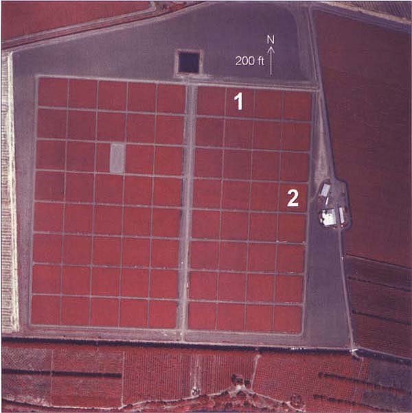
Fig. 1. Color IR photo of the LTRAS site on July 11, 1993, illustrating uniformly managed sudangrass grown to assess variability in soil fertility prior to starting a long-term experiment. Numbers mark two 1-acre plots discussed in text. Arrow indicates orientation and scale.

[View Enlargement]

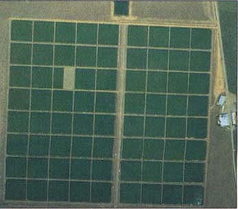
The above photograph is a true-color version of figure 1 at left.

Crop performance may vary considerably within a single field due to spatial differences in such factors as fertility, drainage, soil depth, salinity and root pathogens. Recognition of this within-field variability has led to increased interest in site-specific crop and soil management. For example, it may be possible to match nutrient supply with crop demand at each location within a field by varying fertilizer rate across the field. This could reduce fertilizer costs and the potential for nitrate pollution of groundwater, without reducing crop yield. Mapping areas with poor crop growth may also help farmers to identify and correct yield-limiting factors.

Spatial variability is often a problem in field experiments as well. Large plots minimize errors due to edge effects, but yield estimates based on a small harvested strip within a large plot may not be representative of the entire plot. Variability in soil properties among replicate plots within a treatment can obscure treatment effects. If information on variability within a field is available, it can be used to improve statistical analyses of results. This increases our ability to detect differences among treatments or cultivars that would otherwise be “lost in the variability.” The same information could also be used to identify relatively uniform blocks in the initial layout of a field experiment.

Mapping spatial variability

Both site-specific management and field research would benefit from detailed information on spatial differences in soil properties and crop performance. One possible approach is to divide the entire field into small areas (each perhaps only a few feet square) and to collect a separate soil sample from each. Collecting and analyzing so many soil samples is not usually practical, however, even in research fields. For some crops, yield monitors are now available that can be attached to a harvester to record the amount of material, such as grain, harvested every few seconds. These yield monitors are typically used with a satellite-based global positioning system to generate a detailed map of yield patterns across the field. Growers can refer to the yield map for site-specific management in subsequent years, assuming that the yield-limiting factors do not change from year to year. Although yield mapping is a promising new technology, it is not yet in widespread use in California.

Color infrared (IR) aerial photography is a relatively mature technology that may also be useful for mapping variability within a field. Aerial photography has some potential advantages relative to other detailed mapping methods. Aerial photos can be taken whenever the weather is clear, including early in the growing season when there may still be time to correct any problems that are identified. It is also relatively inexpensive.

Aerial photography has been used for many years to identify problem spots in fields and vineyards. It has been difficult and time-consuming, however, to obtain meaningful numerical data from aerial photos. This limitation has precluded widespread use of aerial photography for site-specific management and research. An article in the April 1976 issue of California Agriculture suggested that additional information might be obtained in the future by “analyzing infrared photos with sophisticated instruments …” One such sophisticated instrument, a personal computer equipped with slide scanner and image processing software, is now widely available. We therefore decided to explore the potential of these new tools for analyzing infrared aerial photos of field crops.

From field to computer screen

All color IR photos were taken with a Maurer P-2 camera with a 76 mm lens covered with a yellow filter (equal to a Tiffen #8). Shutter speed was 1/500 second and aperture varied from f-5.6 to f-8, depending on season and lighting conditions. Format was 2 1/4 x 2 1/4 inches using 70 mm film (Kodak Aerochrome 2443). The 70 mm transparencies were scanned with a slide scanner. The resulting TIF-format computer file had a spatial resolution of 1200 x 1200 pixels, with 24 bits per pixel (8 bits x 3 colors).

Figure 1 is an example of a scanned color IR aerial photo. The photo, which was taken on July 11, 1993, from 4,000 feet above the UC Davis Long Term Research on Agricultural Systems (LTRAS) site, illustrates a sudan hay crop just prior to harvest. This uniformly managed “time zero” crop was grown to assess variability within and among plots prior to initiating experimental treatments in a 100-year experiment at the site.

Note that the colors in color infrared photos do not correspond to true colors in the field. For example, near IR wavelengths are shown as red. Healthy green leaves reflect near IR strongly and therefore appear red in IR photos.

Vegetation index

Some qualitative differences are apparent within and among the plots in figure 1 (compare the plots labeled 1 and 2), but it is difficult to make quantitative comparisons. To obtain numerical data useful for site-specific management or field research, the scanned image was therefore processed using the software package Image Pro for Windows (Media Cybernetics, Silver Spring, MD).

First, the scanned image was aligned with four ground reference points. This operation corrected for differences in the flight path of the airplane and facilitated comparisons among photos taken on different dates. Then the Image Pro software was used to calculate the Normalized Difference Vegetation Index (NDVI), defined as the difference between the IR and red values for each pixel, divided by their sum.

This NDVI formula, NDVI = (IR-red)/(IR+red), is based on the fact that healthy leaves reflect near-infrared light while absorbing red light. Larger values of NDVI indicate either more complete coverage of the ground by leaves or differences in leaf spectral properties. The three numerical values associated with each pixel in the image (representing reflectance of IR, red and green light) were replaced with a single NDVI value calculated from the IR and red values for that pixel. (Because near-IR and red are displayed as red and green, respectively, in color IR photos, the software uses values for the “red” and “green” bands.) NDVI is widely used in satellite imaging (see Applications of Remote Sensing in Agriculture, ed. M.D. Steven and J.A. Clark, Butterworths, 1990, for examples), but we are not aware of any published accounts of its use with aerial photos. Other vegetation indices, such as the simple ratio of IR to red, may also be useful.

Characterizing the LTRAS site

Figure 2 presents NDVI values calculated from the color IR image illustrated in figure 1. Differences in NDVI values among plots appear as differences in color, with the lowest values represented by black and the highest values represented by white. NDVI values were correlated with subsequent hay yields for each plot (fig. 3A). Both hay yields and NDVI values were lowest in areas where the most topsoil was removed during initial leveling of the field—for example, along the west (left) edge. Three low-yielding plots are not being used in the main 100-year LTRAS experiment. Although NDVI was correlated with hay yield, leaf area of this mature crop (over 5 feet high) was great enough in all plots to cover the ground almost completely. Differences in NDVI may therefore reflect differences in leaf spectral properties (possibly related to leaf chlorophyll content) rather than differences in leaf area in this case.

[View Enlargement]

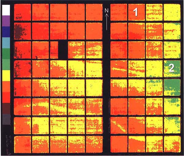
Fig. 2. Normalized Difference Vegetation Index (NDVI) calculated from figure 1. NDVI scale ranges from 0 (black) to 1 (white). A contrast-enhanced version of this figure appears on the cover.

Lingering effects of an old water channel are also visible in figure 2, running roughly from west to east. This channel was presumably backfilled with topsoil during land leveling, which could explain the higher NDVI value relative to neighboring areas.

Figure 4 presents NDVI values on March 8, 1994, for the first winter crops grown at LTRAS. Only the northeast corner of the field is shown. Wheat plots receiving nitrogen fertilizer (F) had greater leaf area (or higher chlorophyll content) than unfertilized wheat (U). Legume cover-crop plots (CC), which relied on biological nitrogen fixation rather than synthetic fertilizer, had NDVI values more similar to fertilized than to unfertilized wheat. At the elevation used in figure 4 (2,000 feet), each pixel corresponds to an area approximately 2 feet on a side. The 70 mm negative could be scanned at higher resolution if even more detail were needed.

[View Enlargement]

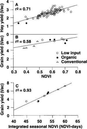
Fig. 3 (A). Relationship between NDVI and hay yield for each plot shown in figure 2. Solid symbols (2 overlap) indicate 3 plots not used for the long-term experiment because of unusually low NDVI and yield; (B) Relationship between NDVI on August 1, 1994, and subsequent corn grain yield at SAFS; (C) Relationship between NDVI (integrated over growing season) and corn grain yield at LTRAS. Symbols as in B, but cropping systems at SAFS and LTRAS are not identical.

[View Enlargement]

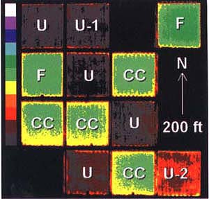
Fig. 4. Northeast corner of LTRAS site (see figs. 1 and 2) illustrating NDVI of winter wheat and legume cover-crop plots on March 8, 1994. U = unfertilized wheat, F = fertilized wheat, CC = cover crop. Each pixel corresponds to an area approximately 2 feet on a side. NDVI ranges from 0 (black) to 1 (white).

Figure 4 illustrates the value of doing initial site characterization prior to a long-term field experiment. Plots U-1 and U-2 were both managed identically, yet there was a substantial difference in NDVI (and subsequent grain yield) between them. At least part of this difference may be explained by initial differences in soil quality, as indicated by differences in NDVI of the initial (“time zero”) sudangrass crop (fig. 2). By including these time-zero data as a covariate in our statistical analyses, we were able to detect subtle differences among treatments even in the early years of this long-term experiment.

Edge effects are also apparent in figure 4. Within the unfertilized wheat plots, improved growth occurred along the north and south edges, whereas legume cover-crop plots and fertilized wheat plots had better growth in the center than at the edges. These edge effects were also apparent to observers in the field as differences in height or leaf color. The positive edge effects in the unfertilized plots may have resulted from nutrient-rich runoff from the field roads between the plots. The reason for the negative edge effects in the fertilized and cover-crop plots is not known. Water stress or differences in irrigation could be a factor at other times of the year, but neither explanation applies to this image from early March. Cover crop plots at LTRAS have never been irrigated.

[View Enlargement]

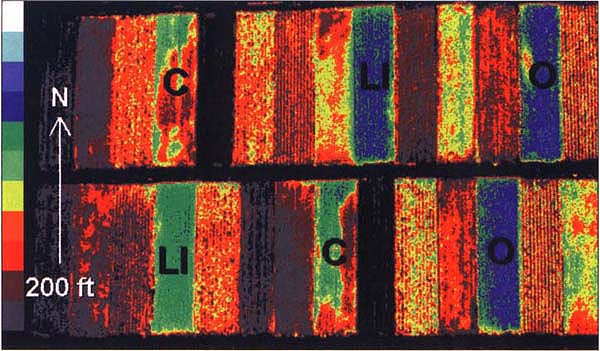
Fig. 5. NDVI at SAFS on August 1, 1994. Conventional (C), low-input (LI) and organic (O) corn plots are indicated. NDVI ranges from 0 (black) to 1 (white).

In the 1-acre plots used at LTRAS, these edge effects affected only the 50-foot border of each plot, which was not used for yield measurements. Edge effects could have greater effects on yield estimates for smaller plots, which often use unsampled borders (if any) of only a few feet. Based on figure 4, we predict that yield estimates from small plots would overestimate the productivity of unfertilized wheat and underestimate that of legume cover crops or fertilized wheat.

Several of the unfertilized wheat plots illustrated in figure 4 are actually the first year of a 2-year rotation with a winter-legume cover crop. The effects on wheat yields of substituting a cover crop for the fallow year will be seen in subsequent years. The other unfertilized plots were included as a control, to allow the nitrogen supply from soil organic matter, rainfall and other natural (intrinsic) sources to be estimated.

Corn growth at LTRAS and SAFS

Corn is included in rotations both at LTRAS and in the Sustainable Agriculture Farming Systems (SAFS) experiment, also at UC Davis. Although none of the cropping systems at SAFS correspond exactly to those at LTRAS, a comparison of roughly comparable systems is interesting. Data for SAFS presented here are for the sixth year of this 12-year experiment, whereas LTRAS data are for the first year of a 100-year experiment. For more information on SAFS cropping systems, see the September-October 1994 issue of California Agriculture.

At SAFS, corn in the conventional system (C) had lower average NDVI values than either organic (O) or low-input (LI) corn on August 1, 1994 (fig. 5). Conventional corn plots at SAFS also showed marked within-plot nonuniformity in NDVI. Average grain yields were also lower in the conventional plots, and yields were significantly correlated with NDVI measured on August 1, 1994 (fig. 3B). Leaf chlorophyll at silking (measured using a Minolta SPAD 201 chlorophyll meter) was lower in the conventional corn, relative to the other systems. The poor performance of the conventional corn at SAFS might be explained by problems with irrigation water infiltration in the conventional plots. Winter cover crops and supplemental manure inputs over the first 6 years of the experiment may have improved soil structure and infiltration of irrigation water in the organic and low-input systems, relative to the conventional system. Additional data pertaining to this question have been submitted to Agronomy Journal.

An IR aerial photo taken at LTRAS on the same day reveals a very different pattern. All corn plots had similar NDVI values (uniformly green plots in fig. 6) on August 1, 1994. (Absolute values of NDVI may not be comparable between figures 5 and 6 because the photo of SAFS was taken from an elevation of only 1,650 feet versus 4,000 feet at LTRAS. Calibration panels with standard reflectance values could be included in future photos to facilitate absolute comparisons.)

Earlier in the season there were significant differences among corn plots at LTRAS, but the treatment effects were not consistent with those at SAFS. On June 13, 1994, for example, conventional corn plots at LTRAS had higher average NDVI than organic plots, which in turn had higher NDVI than “low-input” plots with the winter-legume cover crop as sole nitrogen input (fig. 7). At LTRAS, conventionally managed corn (C) was seeded on April 14, 1994, and fertilized with a seasonal total of 270 lb N/acre. Organic (O) and low-input corn (L) were both seeded on May 5, 1994, following incorporation of a winter legume cover crop (Lana woollypod vetch mixed with Austrian winter peas) containing 180 lb N/acre on April 1, 1994. The organic corn also received 8 tons/acre of composted poultry manure (3.7% N), or 590 lb N/acre. The organic plots therefore received nearly three times as much total N as the conventional plots, because we assumed that only 30 to 40% of the N in these organic sources would be available during the first year. Soil nitrate during grainfill did not exceed 5 ppm (?g/gDW) in either system.

Although all three systems eventually achieved full cover (fig. 6), total seasonal photosynthesis was presumably limited in the alternative systems by less leaf area early in the season (for example, fig. 7). Correlations between yield and total seasonal light interception have been reported for many crops (J. L. Monteith, Agricultural and Forest Meteorology 68:213-220). We do not yet have any data on the exact relationship between NDVI and the fraction of sunlight absorbed, but we did find a good correlation (fig. 3C) between corn grain yield and integrated seasonal NDVI — that is, the area under a curve for NDVI over the growing season. The NDVI curve was based on only three aerial photos during the season, plus seeding and harvest dates.

[View Enlargement]

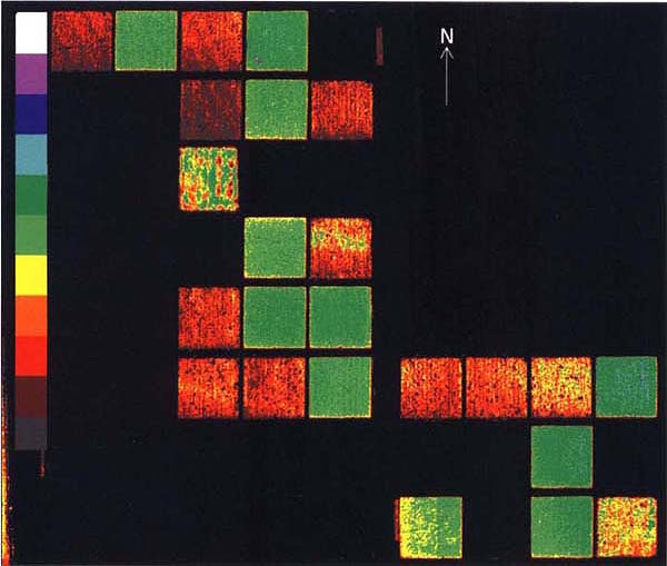
Fig. 6. NDVI at LTRAS on August 1, 1994. All corn plots were uniformly green on this date. Tomato plots (red and yellow) had lower NDVI and were more variable because of incomplete ground cover. NDVI ranges from 0 (black) to 1 (white).

[View Enlargement]

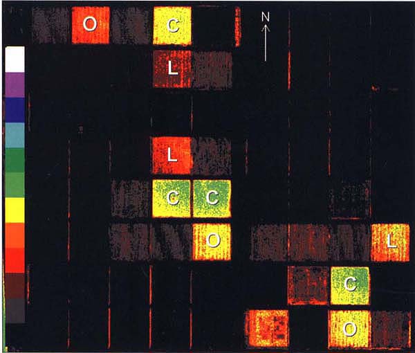
Fig. 7. NDVI at LTRAS on June 13, 1994. Conventional (C), low-input (L) and organic (O) corn plots are indicated. NDVI ranges from 0 (black) to 1 (white).

Much of the yield difference at LTRAS presumably resulted from earlier seeding of conventional corn relative to the alternative systems. The time required for growth, incorporation and partial decomposition of the cover crop will usually result in at least some delay in seeding of corn after a winter legume. On the other hand, the advantages of early seeding in the conventional system could be outweighed by poor infiltration of irrigation water if problems similar to those at SAFS develop in the conventional plots at LTRAS over the next few years of this 100-year experiment.

Computer processing of scanned IR aerial photos is now easy to accomplish with appropriate software. The Normalized Difference Vegetation Index (NDVI) can reveal differences in plant growth and health that are difficult to see in the original color IR image and can provide quantitative information appropriate for site-specific management. NDVI values for a single date may or may not be correlated with final yield (compare figs. 5 and 6). Integrated seasonal NDVI can be a more useful predictor of yield than values for a single date.

Return to top