


All Issues
Wine grape establishment and production in southern California
Publication Information
California Agriculture 44(5):36-37.
Published September 01, 1990
PDF | Citation | Permissions
Abstract
An economic study of vineyard costs in the major wine grape production area of southern California indicates that establishment and production costs exceed returns.
Full text
During the 1970s and early 1980s, Rancho California developed into southern California's main grape production area. Since 1970, wine grapes there have increased from 29 to 2,820 acres. However, local growers are still asking questions about capital outlays and profitability as they consider future expansion and redevelopment.
The purpose of this project was to determine the profitability of investing in a vineyard operation. To measure profitability, I constructed a spreadsheet of vineyard development costs and then altered price and yield parameters to determine the resultant profits. Costs were obtained by a 1988 mail survey and follow-up interviews in person and by telephone with growers, owners, management companies, and dealers in southern California, particularly the Rancho California area. The specifications making up the basis of this profitability analysis follow.
Specifications
Costs were standardized for a 50-acre, owner-operated vineyard to approximate the most common situation in the area. The typical varietal mix included 30 acres of Chardonnay, 10 of Sauvignon Blanc, 5 of Chenin Blanc, and 5 acres of other varieties.
A bilateral cordon training system with 450 plants per acre was used for all varieties. No varietal differences were considered in the cultural practices, since most practices are common to all varieties.
Yields for the varieties commonly ranged from 4 to 8 tons per acre. Using a weighted average, I estimated a single yield of 5 tons per acre for the specified vineyard.
Prices for varieties ranged from $200 to $800 per ton. The weighted average price was $617 per ton.
Using drip irrigation, the annual per-acre water application was 0.25 acre-foot for the first to third years and 1.50 acre-feet for the fourth year on. Water cost varied from $187 to $403 per acre-foot, depending on elevation. This study assumed a water charge of $275 per acre-foot, the charge for a medium-sloped vineyard.
Wages for labor, including fringe benefits, were $5.35 per hour for manual labor and $7.45 per hour for machinery labor.
The interest charge on operating capital and machinery investment was 11.5%, the most common rate for short-term and intermediate loans in 1988.
Management charges were not included, since most surveyed farms did not provide this information and the widely varying wages and salaries for professional managers made it difficult to approximate a typical situation. After all the costs are subtracted from the receipts, the return to management and risk remains as a residual.
All land is assumed to be owned by the operator. Thus, property tax was $11.30 per $1,000 of land value. The values for the specified medium-sloped land ranged from $7,000 per acre for open land to $13,000 per acre for a matured vineyard.
Land rent was imputed using opportunity cost. A 13% investment charge was applied to the value of open land. This rate approximates the cost of capital on real estate loans charged by most federal land banks in the area in 1988.
Establishment costs were amortized at 13% over 25 years, a period corresponding to the expected economic life of grapevines. Uncertainty about future prices, yields, technology, and inflation rates affects the estimates of net cash revenues and terminal values of investments. These estimates become more difficult for investments with longer lives, because more distant events are more difficult to predict. Thus, amortization was at a higher rate than interest on shortterm and intermediate investments. Higher discount rates could mean understated profitability, but they provide a margin for error in estimating net cash revenues under risk.
Cost analysis
The summary of costs, broken into variable, fixed, and total costs, is presented in table 1. For any year, the variable category includes all costs for material, machinery repair, fuel and lubrication, interest on operating capital, and labor. The fixed costs are depreciation, interest, insurance, taxes and housing on machinery investment, rent and property taxes on land, and investment amortization.
The overall cost estimate indicated a $12,066-per-acre establishment cost. The costs are split between variable (40%) and fixed (60%). Fixed costs have an important influence on establishment costs.
Two of the fixed-cost items are particularly significant. The land rent accumulating to $3,640 per acre accounted for 30% of the total establishment cost. Investment amortization accumulating to $2,102 per acre accounted for 17% of the total establishment cost. Together, those two items amounted to $5,742 per acre, accounting for almost half of the total establishment costs.
The annual production cost estimate from year 5 on was $3,891 per acre (table 1). The variable and fixed costs split 34 and 66%, respectively, again reflecting the major role that fixed costs played on costs and profits. Here again, land rent and investment amortization together amounted to $2,219 per acre, 57% of total production costs (table 2).
Profitability analysis
Break-even analysis was performed by ranging price and yield parameters in the cost model described above. The results of the analysis are shown in figure 1. In the figure, gross returns at various price and yield combinations are presented by the upward trending successive lines, and costs are presented by the horizontal lines. The lower horizontal line represents the variable cost, and the upper horizontal line represents the total cost. The break-even points occur where the horizontal (cost) lines cross the gross return lines.
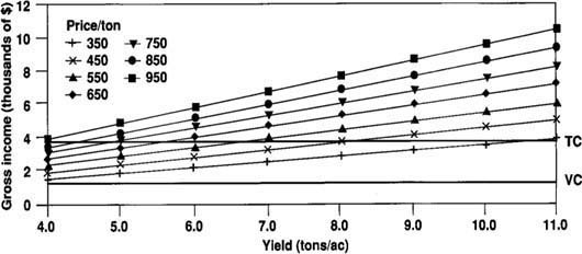
Fig. 1. Break-even analysis of wine grape production at various prices and yields. The two horizontal lines represent variable costs (VC) and total costs (TC). Growers can break even when their gross income for a given tonnage at a given price exceeds their total costs.

TABLE 1. Summary of per-acre establishment and production costs, wine grape vineyard, Rancho California, 1988 (based on 50-acre vineyard)
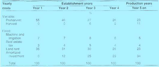
TABLE 2. Percentage breakdown of per-acre establishment and production costs, wine grape vineyard, Rancho California, 1988 (based on 50-acre vineyard)
Figure 1 shows that the yield and price levels for 5 tons per acre and $617 per ton were sufficient to cover variable costs, but not to cover total costs. Excluding harvest costs, estimated total cost break-even points included a yield of 52/3 tons per acre with the price held constant at $617 per ton, or a price of $695 per ton with the yield held constant at 5 tons per acre. Adding in harvesting costs, break-even points rise to 61/2 tons per acre, or $780 per ton at 5 tons per acre. For this investment to be profitable, an increase in either or both parameters (yield and price) must be attained. Using figure 1, growers can test various possible combinations of price and yield for break-even points and profitability.
Investment analysis
Investment analysis on the 50-acre vineyard was based on net present value (NPV) and the internal rate of return (IRR). NPV is the sum of all possible net earnings of the investment discounted into the present value.
Using a simulation model to select yields and price variations at random from a 13-year production record, net earnings for several years were calculated as follows. First, taxable incomes were calculated as gross returns minus operating costs and depreciation. Second, income taxes were determined based on the 1988 tax rate for regularly taxed corporations. Third, the net earnings were determined by subtracting the operating costs and income taxes from gross receipts. (If there are cash receipts from the sale of assets, they should be added to this figure. No cash receipt information was available in this study.)
By compounding the net earnings at discount rates ranging from 6 to 10%, I arrived at the NPVs in table 3. The NPVs were negative at discount rates of 7% and above.
From table 3, we can see that the IRR, the discount rate that makes the present value of the net earnings just equal to zero, lies between 6 and 7%. The exact rate extrapolates to approximately 6.62%. In other words, the IRR is smaller than all the opportunity costs of capital used in the study. If we assume that the owner is a profit maximizer, the development of a vineyard would be unprofitable. This rate can also be interpreted as the break-even rate that equates the present value of cash inflows with cash outflows.

The important point is that IRR is a measure of the productivity of asset use that allows a comparison with returns offered in other uses (i.e., opportunity costs).
Conclusion
Given this scenario of vineyard size, varietal mix, and location, the estimated costs of carrying the establishment cost into the full production years gave an annual production cost of $3,892 per acre. The gross returns estimate, on the other hand, was $3,085 per acre, $806 less than the cost of production. To break even, the operator would have to get $780 per ton at 5 tons per acre yield, or $617 per ton at 61/2 tons per acre yield.
Because no management charges were included in the total costs, higher returns must be attained through increased yield, improved prices, or a combination of the two. Based on the gross returns scenario (fig. 1), various possible combinations of price and yield can be tested for break-even points and profitability.
Different operations used different accounting procedures and cost estimation techniques. Furthermore, the use of imputed costs in agriculture generally has posed both conceptual and estimating problems, resulting in varying degrees of importance being given to the use of imputed costs in profit analyses by farm operators. The conclusion that costs exceed returns should be understood in the following context:
The owner-operator will consider the profitability of crop production relative to other activities, and impute all opportunity costs or foregone returns along with the usual production expenses. We found that imputed costs can significantly impact the costs and profitability as reflected in the fixed costs. Of particular significance are the annual amortization and land rent charges, which accounted for almost 50% of the establishment and 57% of the annual production costs. The overall fixed cost contribution to the establishment and production costs exceeded 60%.
The study did not address the situations of all vineyard operations in the Rancho California area. However, the methodology used to analyze costs, profits, and investments is important to those contemplating expansion or new investment in wine grape production.
Wine grape establishment and production in southern California