


All Issues
Remote sensing is a viable tool for mapping soil salinity in agricultural lands
Publication Information
California Agriculture 71(4):231-238. https://doi.org/10.3733/ca.2017a0009
Published online April 07, 2017
Abstract
Soil salinity negatively impacts the productivity and profitability of western San Joaquin Valley (WSJV) farmland. Many factors, including drought, climate change, reduced water allocations, and land-use changes could worsen salinity conditions there, and in other agricultural lands in the state. Mapping soil salinity at regional and state levels is essential for identifying drivers and trends in agricultural soil salinity, and for developing mitigation strategies, but traditional soil sampling for salinity does not allow for accurate large-scale mapping. We tested remote-sensing modeling to map root zone soil salinity for farmland in the WSJV. According to our map, 0.78 million acres are salt affected (i.e., ECe > 4 dS/m), which represents 45% of the mapped farmland; 30% of that acreage is strongly or extremely saline. Independent validations of the remote-sensing estimations indicated acceptable to excellent correspondences, except in areas of low salinity and high soil heterogeneity. Remote sensing is a viable tool for helping landowners make decisions about land use and also for helping water districts and state agencies develop salinity mitigation strategies.
Full text
Soil salinity is a known constraint on agricultural production in the Central Valley, particularly in the western San Joaquin Valley (WSJV), where soils are naturally high in salts due to the marine origin of their Coastal Range alluvium parent material (Letey 2000). In such a large region, it is difficult to quantify and map the full extent of soil salinity and its impact on agricultural production and profits. Many geological, meteorological and management factors affect the salinity levels of irrigated soils, including irrigation water quality, irrigation management, drainage conditions, rainfall and evapotranspiration totals and cultural practices. Across a region such as WSJV, most of those factors vary at multiple spatial and temporal scales, making it difficult to extrapolate local point measurements of soil salinity to regional scales.
Although agricultural salinity is a generally well-known issue, communicating the full extent and severity of the problem to policymakers, stakeholders and other nonspecialists is a challenge. Detailed regional maps present the problem visually and can help spur action on planning, management and conservation. Letey (2000) argued that long-term sustainable and profitable agriculture in California can be achieved only if regional-scale salt balances can be obtained. Regional-scale salinity maps provide irrigation district managers, water resource specialists and state and federal authorities with timely information that can guide decisions on water allocation needs and groundwater regulation.
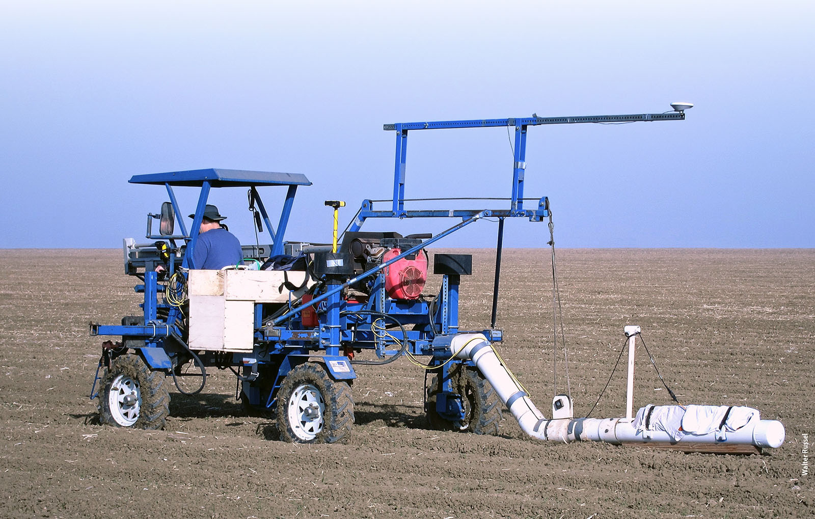
This electromagnetic induction rig was developed at the USDA-ARS U.S. Salinity Laboratory for mapping soil salinity and other soil properties (e.g., texture, water content, bulk density, organic matter) at field scale. Regional-scale salinity maps provide irrigation district managers, water resource specialists and state and federal authorities with timely information that can guide decisions on water allocation needs and groundwater regulation.
Remote sensing of soil salinity
In the past decade, efforts to map soil salinity at regional scales and characterize its spatial variability have focused on the use of predictor covariates that can be observed remotely with continuous spatial coverage across a region (e.g., Lobell et al. 2007). Remote sensing is ideal for identifying within-field variability, which is known to exist in the farmland of the WSJV (e.g., Lesch et al. 1992). This remote-sensing approach is in contrast to traditional methods of assessing soil salinity by soil sampling, which are typically carried out at coarse resolution (e.g., soil samples every ∼ 1,000 to 1,500 yards). In their recent soil survey reports (e.g., Arroues 2006), the Natural Resources Conservation Service (NRCS) provided salinity estimations only for nonirrigated soils because the influence of irrigation on soil salinity cannot be accounted for at the regional scale using traditional soil survey protocols. Remote sensing, however, is able to capture abrupt changes between neighboring fields that have the same soil type but are managed differently (fallow vs. irrigated, drip vs. flood irrigation).
In discussing remote sensing of saline soils, one must distinguish between salinity at the soil surface (sometimes visible as salt crusts) and salinity in the soil root zone (i.e., the soil volume down to a depth of about 3 to 5 feet). Soil root zone salinity affects plant growth, and it is the salinity indicator of greatest interest in agricultural assessments.
When a crop is stressed by root zone salinity, an increase in crop reflectance occurs in the blue (B), green (G) and red (R) ranges of the electromagnetic spectrum (e.g., leaves turn from green to hues of yellow and/or red), and a decrease occurs in the near-infrared (NIR) range. Recent research suggests that root zone salinity can be determined indirectly based on canopy reflectance measurements (Lobell et al. 2010; Zhang et al. 2011). Specifically, vegetation indices such as the Normalized Difference Vegetation Index (NDVI) or the Canopy Response Salinity Index (CRSI), calculated from satellite multispectral reflectance data, can be used to infer root zone salinity within a satellite image pixel. Unfortunately, other stressors such as pests and agronomic mismanagement have similar effects on crop reflectance. Thus, it is necessary to devise a procedure for separating the effects of salinity from other stressors.
Whereas most stressors tend to fluctuate within years and from year to year, average root zone salinity is relatively stable assuming consistent farming practices (Lobell et al. 2010). Scudiero et al. (2015) hypothesized that over a period of 5 to 7 years, the year of maximum plant performance (biomass production) as indicated by plant reflectance values would correspond to a time when transient stressors were minimized and salinity stress would be most clearly observable. Scudiero et al. (2015) developed a prediction model for WSJV root zone salinity using CRSI as a predictor variable. The CRSI is defined (Scudiero et al. 2014) as

Increased plant vigor corresponds to a higher CRSI value. Notice that the CRSI is not a salinity-specific vegetation index; it was selected by Scudiero et al. (2015) because it provided better performance than other vegetation indices when applied to their salinity ground-truth calibration data.
Scudiero et al. (2015) calculated CRSI values using Landsat 7 ETM+ canopy reflectance data with a resolution (pixel size) of 32.8 × 32.8 yards (900 square meters). The pixel root zone (∼ 0 to 4 feet) salinity prediction model of Scudiero et al. (2015) for 2007 to 2013 is
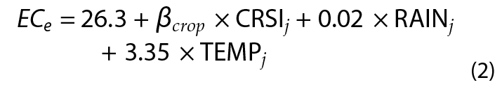
where: ECe is soil salinity (deciSiemens per meter, dS/m, see Box 1), the subscript j indicates the year of the maximum CRSI value, RAIN (mm) is the total rainfall for the year and TEMP (°C) is the average daily minimum temperature for the year. Scudiero et al. (2015) considered various predictor variables and equation formulations before selecting equation 2. Meteorological data were evaluated and included in the model because of their known effects on plant growth. The βcrop parameter indicates the presence or absence of cropping and has a value of −100.76 for fallow soils and −93.40 otherwise.
Box 1. Laboratory measurement of soil salinity
Soil salinity is quantified as the electrical conductivity of a saturated soil paste extract (ECe, dS/m). The United States Salinity Laboratory (Richards 1954) classifies agricultural ECe in these categories: 0 to 2 dS/m (nonsaline), 2 to 4 dS/m (slightly saline), 4 to 8 dS/m (moderately saline), 8 to 16 dS/m (strongly saline) and > 16 dS/m (extremely saline).
Scudiero et al. (2015) calibrated the model using data for 5,283 Landsat 7 pixels located in 22 WSJV fields that had been extensively surveyed for salinity by Scudiero et al. (2014). The model calibration produced R2 = 0.73. Scudiero et al. (2015) cross-validated the model with traditional k-fold resampling (k = 22), yielding an observed-predicted R2 of 0.68, and with a more conservative spatially independent leave-one-field-out (lofo) resampling (R2 = 0.61). In particular, the lofo resampling indicated that the mean absolute error (MAE) at unknown fields is expected to be: 2.94 dS/m (nonsaline), 2.12 dS/m (slightly saline), 2.35 dS/m (moderately saline), 3.23 dS/m (strongly saline) and 5.64 dS/m (extremely saline). See Box 1 for definitions of soil salinity classes. Further details on remote-sensing data processing, model development and cross-validation statistics are provided in Scudiero et al. (2015).
For this article, we used the calibrated equation 2 to generate a salinity map for the WSJV. Our goals were to reveal the extent and spatial distribution of salinity across the WSJV and consider the accuracy and possible limitations of the map. We also wanted to explore how remote sensing of soil salinity can be used to support agriculture in California.
WSJV salinity map
Figure 1 shows the remote-sensing root zone salinity map for the WSJV with a resolution of 32.8 × 32.8 yards. The map was generated from equation 2 using spatial input data from 2007 to 2013 — Landsat 7 EMT+ reflectance data, PRISM model meteorological data (Daly et al. 2008) and CropScape (Han et al. 2012) cropping data. Nonagricultural areas (e.g., urban land, water bodies, roadways) were masked. Orchards were also masked because the dataset used by Scudiero et al. (2015) to calibrate equation 2 did not include tree crops. According to the CropScape database, 16.2% of WSJV farmland was cropped with orchards in 2013. Later in this article, we discuss remote-sensing mapping over orchards.
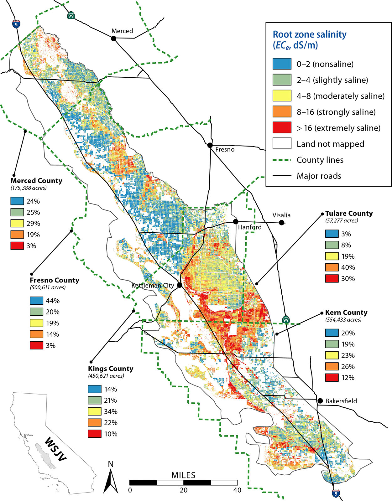
Fig. 1. Remote-sensing estimations of root zone (0 to 4 feet) soil salinity for agricultural soils (orchards not included) of the west side of the San Joaquin Valley (WSJV). Boxes indicate the extent (in percentage) of soil salinity in the five counties of the WSJV.
According to our map (fig. 1), 0.78 million acres are salt affected (i.e., ECe > 4 dS/m), which represents 45% of the mapped farmland. The mapped acreage for the different subclasses of soil salinity were 433,777 acres (25%) nonsaline, 349,007 acres (20%) slightly saline, 436,476 acres (25%) moderately saline, 374,000 acres (22%) strongly saline and 145,070 acres (8%) extremely saline. Figure 1 shows breakdowns for individual counties (Merced, Fresno, Kings, Tulare and Kern).
Remote-sensing map accuracy
Scudiero et al. (2015) found good model accuracy when equation 2 was tested using various forms of cross-validation on a large ground-truth dataset representing 22 WSJV fields and thousands of remote-sensing pixels. Compared to that dataset, however, figure 1 represents a substantially greater application of . Although extensive data for assessing the accuracy of the WSJV map do not exist, some limited evaluation of the map accuracy is possible, because some of the image and landscape variables that influence the accuracy are known.
Independent salinity measurements
Figure 2 compares the salinity estimated using equation 2 over ∼ 4,000 acres (1,619 hectares) of farmland in Lemoore (Kings County) with independent salinity measurements made on 25 soil cores that were sampled in 2011 and 2012 by Wang (2013). According to the NRCS Soil Survey Geographic database (SSURGO), texture in this area is fairly uniform (clay and clay loam, mostly). The independent soil measurements are sparse point data (2-inch-diameter cores) that cannot be usefully compared with the much larger ETM+ pixels. However, since Wang's (2013) soil sampling scheme was not spatially biased (not clustered), the frequency distribution of the independent salinity measurements should be representative of the salinity in the target area (Corwin and Scudiero 2016).
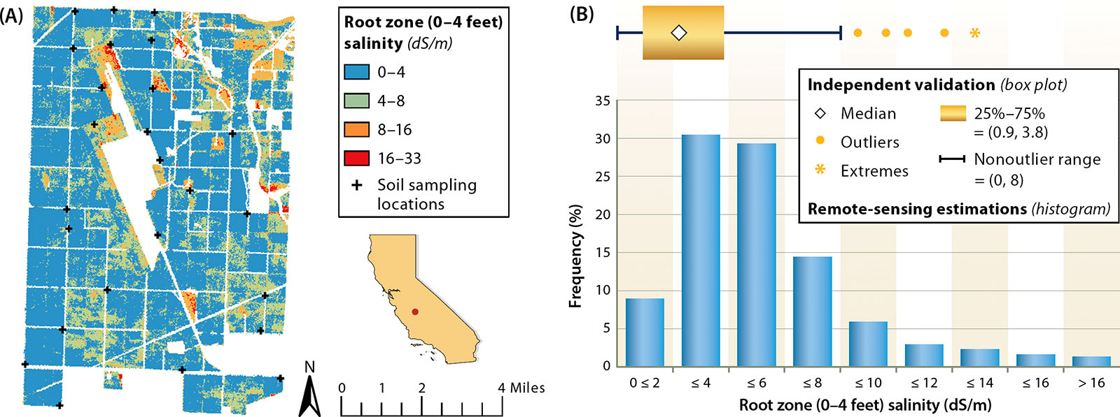
Fig. 2. (A) Remote-sensing estimations of root zone salinity over ∼ 4,000 acres of farmland in Lemoore (Kings County) and (B) the comparison of the remote-sensing estimations frequency distribution with that of independent soil measurements.
The independent soil sampling had an average ECe of 2.8 dS/m (median of 2.3 dS/m and standard deviation of 2.4 dS/m); equation 2 produced a map characterized by an average ECe of 3.2 dS/m (median of 2.5 dS/m and standard deviation of 3.1 dS/m). The similar frequency distributions from the remote-sensing map and independent sampling (fig. 2) indicate acceptable accuracy of the remote-sensing estimations.
Soils with salt crusts
Salt crusts are readily identifiable from remote-sensing imagery (e.g., Metternich 1998). Salt crusts can be seen only on bare soil and have high temporal variability. Although the presence of salt crusts does not necessarily correspond to high root zone salinity, one would expect some correlation to exist (Zare et al. 2015). We qualitatively evaluated the correspondence of remote-sensing high salinity predictions with the presence of salt crusts.
To map salt crusts across the WSJV, we used imagery from the 2014 USDA's National Aerial Imagery Program (NAIP) survey (resolution of 1.09 × 1.09 yards, i.e., 1 square meter). A supervised classification (maximum likelihood classification algorithm) was used to identify salt crusts. The classification identified NAIP pixels with reflectance properties similar to those observed at locations known to be affected by salt crusts. This analysis identified salt crusts over 0.5% of WSJV farmland. Figure 3A depicts a site near Bakersfield (Kern County) where salt crusts are clearly visible in the NAIP ortho-imagery over fallow land but not in the neighboring corn (Zea mays L.) field. There is excellent correspondence between the high salinity (ECe > 8 dS/m) sections of the site as estimated by the remote-sensing map (fig. 3C) and the location of the salt crusts (fig. 3B).
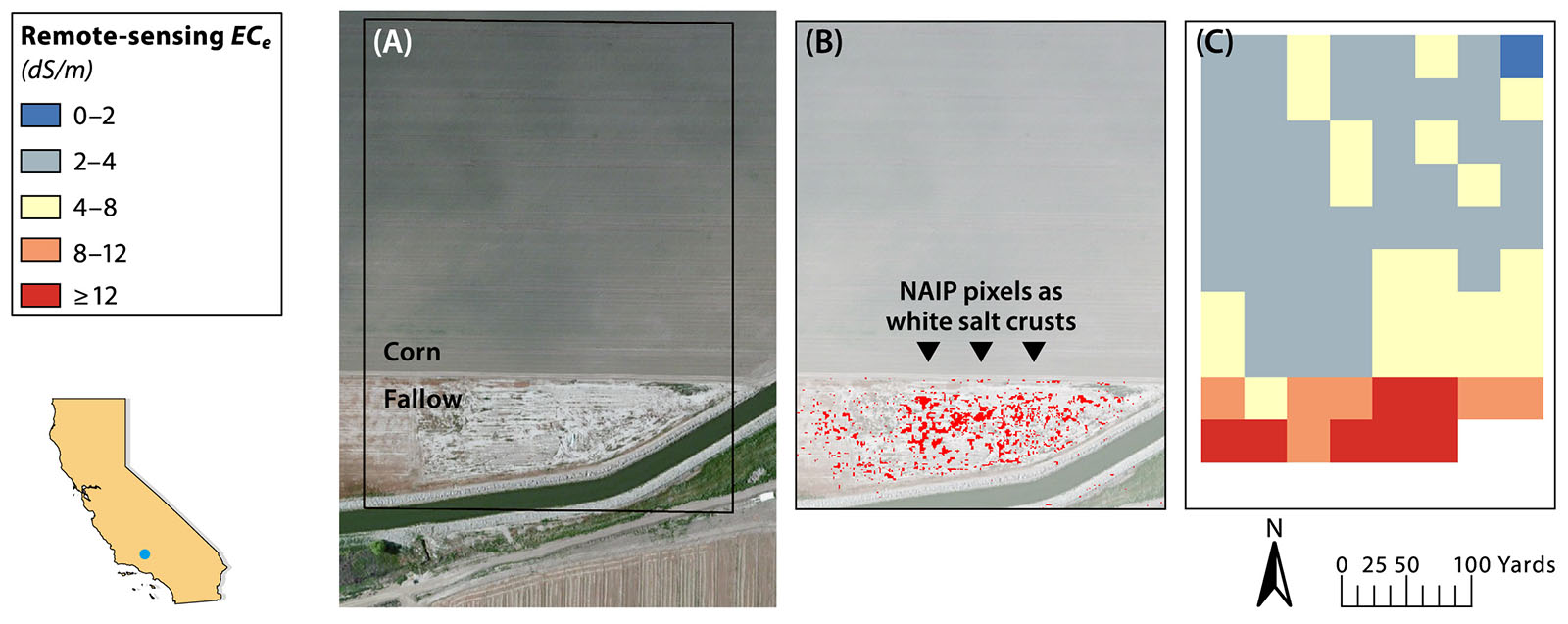
Fig. 3. (A) National Aerial Imagery Program (NAIP) 2014 image of a site in Bakersfield (Kern County), where the field in the north was cultivated with corn (Zea mays L.) and the field in the south was fallow; (B) NAIP pixels classified as white salt crusts by supervised classification (red pixels); (C) remote-sensing estimations for root zone salinity.
To properly compare the NAIP salt pixel classification with figure 1, we aggregated the NAIP classification at the 32.8 × 32.8 yard (30 × 30 meter) resolution. Only the 32.8 × 32.8 yard (30 × 30 meter) cells that included more than 50% of NAIP salt crusts at the original 1.09 × 1.09 yard (1 × 1 meter) resolution were retained for further analysis. A total of 162,829 “salt-crusted” cells were identified. About 94.3% of the salt-crusted pixels were predicted by equation 2 to be ECe > 4 dS/m. In total, the salt-crusted pixels had average ECe of 13.6 dS/m, first quartile of 9.7 dS/m, median of 13.5 dS/m and third quartile of 18.2 dS/m, indicating good correspondence between visibly saline soils and predictions of high salinity by equation 2.
Contrasting soil properties and low salinity
Scudiero et al. (2015) indicated that remote-sensing estimations at low salinity levels (ECe < 4 dS/m) might be imprecise because plants may not be sufficiently osmotically stressed at low salinity to affect crop health. The spatial variability of other soil properties that influence crop yield within a single field could lead to salinity estimation errors at low salinity. Although subfield variations in soil texture are typically minor in WSJV, some fields exhibit significant variability over short distances. In these cases, soil heterogeneity influences crop performance, introducing uncertainty into the remote-sensing estimations of soil salinity.
As an example, consider the remote-sensing salinity predictions for a slightly to moderately saline field located near Stratford (Kings County), along the southern branch of the Kings River. As shown in the NAIP ortho-imagery acquired on July 8, 2003 (fig. 4A), the field is characterized by substantial small-scale soil heterogeneity, which is likely due to movements of the Kings River through paleohistory. The root zone salinity measured by Scudiero et al. (2014) is shown in figure 4B (ground-truth data), and the remote-sensing prediction is shown in figure 4C.
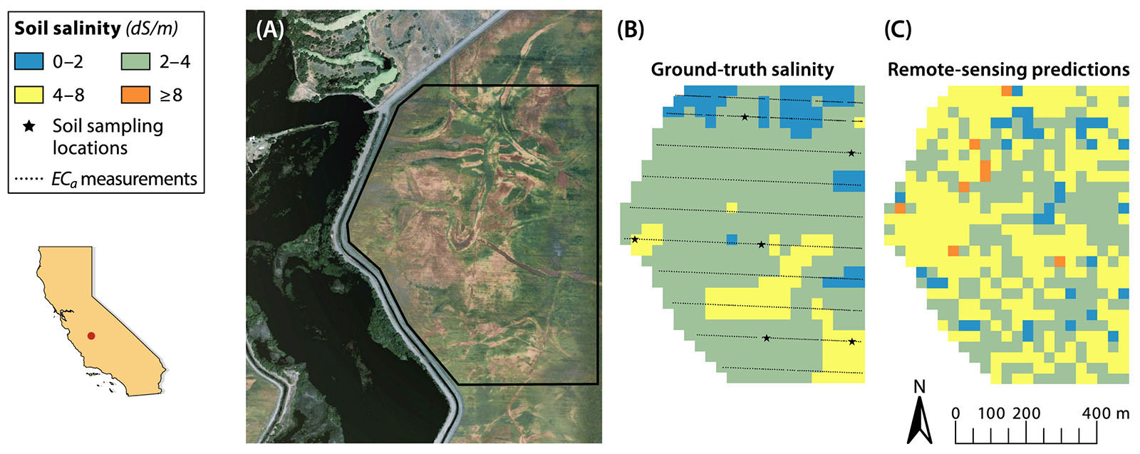
Fig. 4. Example of inaccuracy of remote-sensing estimations in a heterogeneous field with lower salinity values: (A) National Aerial Imagery Program imagery at a test site in Stratford (Kings County) on July 8, 2003; (B) ground-truth root zone (0 to 4 feet) salinity measured by Scudiero et al. (2014) through apparent electrical conductivity (ECa) measurements and soil sampling; and (C) remote-sensing salinity estimations.
In figure 4B, the average ECe was 3.01 dS/m (standard deviation of 0.84 dS/m), whereas in figure 4C the average was 4.22 dS/m (standard deviation of 1.57 dS/m). Clearly, the two maps (figs. 4B and 4C) are not spatially correlated. This is likely due to the confounding effect of soil spatial variability on the salinity estimations. This example shows that when soil salinity is not the only limiting factor for crop production, the spatial patterns of the remote-sensing map might not represent the salinity variations within the target field. This issue can be addressed by including information on soil properties, such as texture, in the remote-sensing model. Unfortunately, at the moment, reliable soil texture maps comparable in resolution to Landsat imagery are not available for California.
Map spatial resolution
High-resolution maps (cell size < 10 yards) can be very useful when planning field agricultural operations, especially when precision farming techniques are employed. The spatial resolution (900 square meters, ∼ 0.22 acre) of Landsat, which was used to produce the remote-sensing salinity map (fig. 1), may seem too coarse to represent within-field spatial variability of soil salinity. However, desired map resolution is not the only factor to consider. When estimating soil properties using remote sensing, one should keep in mind that correlation between soil properties and satellite data might be optimal at coarser resolutions (Gomez et al. 2015; Miller et al. 2015).
A practical example of this can be seen in figure 5. In this 80-acre fallow field near Stratford (Kings County), salinity was mapped with an apparent electrical conductivity survey and soil sampling by Scudiero et al. (2014). Multitemporal (Aug. 22, 2012; Sept. 29, 2012; and April 21, 2013) WorldView-2 (Digital Globe, Colorado) imagery was acquired that has a native resolution of ∼ 2.2 × 2.2 yards (2 × 2 meters). The Enhanced Vegetation Index (EVI) (Huete et al. 2002) was calculated from the imagery, as follows:
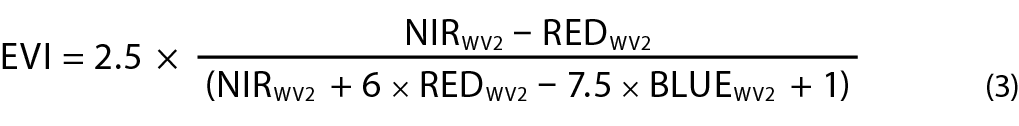
where NIRWV2 (860–1040 nm), REDWV2 (630–690 nm) and BLUEWV2 (450–510 nm) are the WorldView-2 bands employed in the calculation.
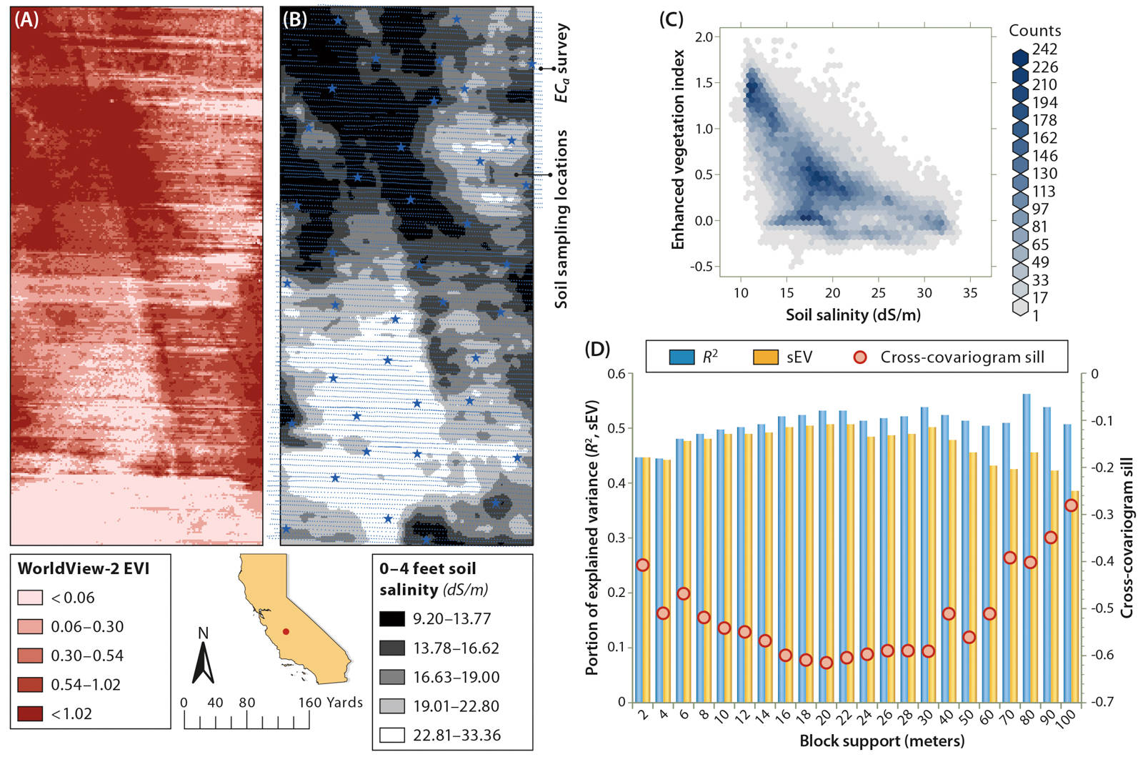
Fig. 5. (A) Enhanced Vegetation Index (EVI) and (B) ground-truth soil salinity (from Scudiero et al. 2014) at 2 × 2 meter resolution for an 80-acre field in California; (C) scatter plot for the two maps; and (D) strength of the relationship at different block supports, measured as coefficient of determination (R2), scaled explained variance (sEV) and a function of the cross-covariogram sill.
The EVI was selected to show that vegetation indices other than CRSI can be used to assess soil salinity, provided they reflect plant status at the target location. The multitemporal maximum EVI map (fig. 5A) from the three WorldView-2 images is visually similar to the ground-truth salinity map (fig. 5B). The two maps are negatively correlated, with a coefficient of determination (R2) of 0.45 (fig. 5C).
Both maps were resampled to coarser resolutions (or block support) to study the changes in the strength of their relationship. As shown in figure 5D, the strength of the salinity-EVI relationship increases as block support decreases. In particular, the scaled explained variance (sEV) and the strength of spatial correlation (see Box 2 for definitions) increase to a maximum at block support of 20 meters (∼ 21.8 yards), then steadily decrease as the resolution becomes coarser. The strength of the salinity relationship with EVI at the Landsat block support (30 meters, ∼ 32.8 yards) was similar to that at 20 meters, indicating that it could properly represent the salinity spatial patterns at this site, despite being slightly coarser than ideal.
Box 2. Quantifying strength of relationships at different spatial resolutions
The variance of a map decreases when it is resampled to coarser resolutions. To compare the relationships between two maps at different resolutions, the coefficient of determination (R2) is not an ideal tool. Indeed, two R2s are comparable only if they refer to the same sample (same variance), which is not the case for maps at different resolutions.
There are two alternative ways of assessing relationships at different scales. The first is using the scaled explained variance: the ratio between variance of predicted salinity at the modeled resolution and variance of observed salinity at the highest resolution. The second is using the cross-covariogram sill: the amount of variance that can be obtained in a prediction (e.g., predicted salinity) by using an explanatory variable (e.g., satellite vegetation index). Practically, the larger the absolute value of the cross-covariogram sill, the stronger the spatial correlation between the studied variables. The cross-covariogram sill is obtained by calculating the theoretical cross-covariance function (Goovaerts 1997) between two spatial variables.
Remote sensing of orchard salinity
Scudiero et al. (2015) focused their research on fields cultivated with annual crops. Their model cannot be applied to orchards, especially young orchards (< ∼ 10 years old). Young orchards have little or no within-row or between-row canopy cover; consequently, the vegetation coverage within a Landsat pixel is low. As an example, figure 6A shows a young 150-acre (60.7-hectare) almond (Prunus dulcis Mill.) orchard in Kern County. At this site, within the selected ETM+ pixel (fig. 6A), the vegetation coverage is low. Soil was sampled at this site at 24 locations in 2013. Figure 6B shows that the remote-sensing model produced overestimates of the salinity at the site. This inaccuracy is likely due to the low canopy coverage. Bare soil reflectance within ETM+ pixels would lower the CRSI values, producing high salinity estimations.

Fig. 6. (A) Independent soil sampling over a 150-acre almond (Prunus dulcis Mill.) orchard in Kern County (B) compared with remote-sensing estimations of root zone salinity.
Given the extent of land farmed with tree crops, future research should focus on developing a remote-sensing model that accounts for partial canopy coverage at these locations. NAIP images could be used to assess the spatial coverage of the tree canopies (and possible presence of cover crops) in order to scale the values of the Landsat vegetation indices to adjust for bare soil reflectance.
Salinity mapping and management
Since the early 1950s, irrigation has played an important role in improving the quality of WSJV soils. As an example, the long-term change in soil salinity for western Fresno County is discussed by Schoups et al. (2005). Schoups and colleagues found that long-term irrigation helped reduce soil salinity across western Fresno County throughout the second half of the 20th century. When irrigation stops, there is a risk that these trends will reverse and that salinity will rapidly increase in lands with shallow groundwater, as observed in the long-term study of Corwin (2012).
Reduced water allocations have caused farmers to use potentially higher salinity groundwater in place of lower salinity surface water and to fallow fields during the ongoing drought. According to the CropScape database, during the drought, fallow land in WSJV increased from an average of 11.8% during the years 2007 to 2010 to 19.2%, 21.0%, 21.6%, 25.9% and 33.7% through the years 2011 to 2015. Land fallowing could lead to increases in root zone salinity, thereby potentially negatively affecting future crop growth in the WSJV (Corwin 2012). When reducing water allocations to farmland, the risks of quick land salinization should be considered.
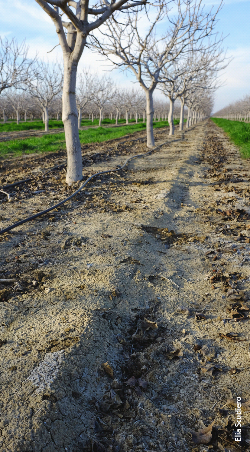
A saline-sodic pistachio orchard near Lemoore showing salt crust present in early winter. Remote-sensing predictions of root zone salinity showed excellent correspondence with the presence of salt crusts.
Updated regional-scale inventories of salinity will provide information for better water management decisions to support statewide agriculture and preserve soil productivity, especially in years of drought, when water resources are limited. With water shortages and droughts likely to become longer and more frequent in the future (Barnett et al. 2008; Cayan et al. 2010), threats from increasing soil salinity are also likely to become more severe and should, therefore, be given serious consideration by landowners, water district managers, and federal, state and local agencies.
Individual soil salinity maps such as presented in this paper can help landowners and water district managers select land they wish to retire or convert to other uses (e.g., solar energy production). But a much greater benefit would be realized if a soil salinity remote-sensing program were established in which maps were created every 5 to 10 years for salinity-affected areas of statewide importance, including the Central and Imperial Valleys. Such a remote-sensing program would allow for the first-time monitoring of soil salinity at regional and state levels, would permit new understandings of drivers and trends in agricultural soil salinity and would aid in the development and assessment of mitigation strategies and management plans.
Remote sensing is a viable tool for mapping soil salinity in agricultural lands